
Why do good predictors end in a p-value of 0.93?
In case you have been following my earlier weblog posts, you may recall that logistic regression encounters an issue when attempting to suit completely separated knowledge, leading to an infinite odds ratio. In Cox regression, the place hazard replaces odds, you may surprise if an identical subject arises with good predictors. It does happen, however in contrast to logistic regression, it’s a lot much less obvious how this happens right here and even what constitutes “good predictors”. As will turn out to be extra clear later, good predictors are outlined as predictors x whose ranks precisely match the ranks of occasion occasions (their Spearman correlation is one).
Beforehand, on “Unbox the Cox”:
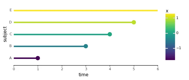
we defined most chance estimation and launched a made-up dataset with 5 topics, the place a single predictor, x, represented the dosage of a life-extending drug. To make x an ideal predictor of occasion occasions, right here we swapped the occasion occasions for topics C and D:
import numpy as np
import pandas as pd
import plotnine as p9from cox.plots import (
plot_subject_event_times,
animate_subject_event_times_and_mark_at_risk,
plot_cost_vs_beta,
)
perfect_df = pd.DataFrame({
'topic': ['A', 'B', 'C', 'D', 'E'],
'time': [1, 3, 4, 5, 6],
'occasion': [1, 1, 1, 1, 0],
'x': [-1.7, -0.4, 0.0, 0.9, 1.2],
})
plot_subject_event_times(perfect_df, color_map='x')
To know why these “good predictors” will be problematic, let’s choose up proper the place we left off and verify the unfavorable log-likelihood value plotted in opposition to β:
negloglik_sweep_betas_perfect_df = neg_log_likelihood_all_subjects_sweep_betas(
perfect_df,
betas=np.arange(-5, 5, 0.1)
)
plot_cost_vs_beta(negloglik_sweep_betas_perfect_df, width=0.1)
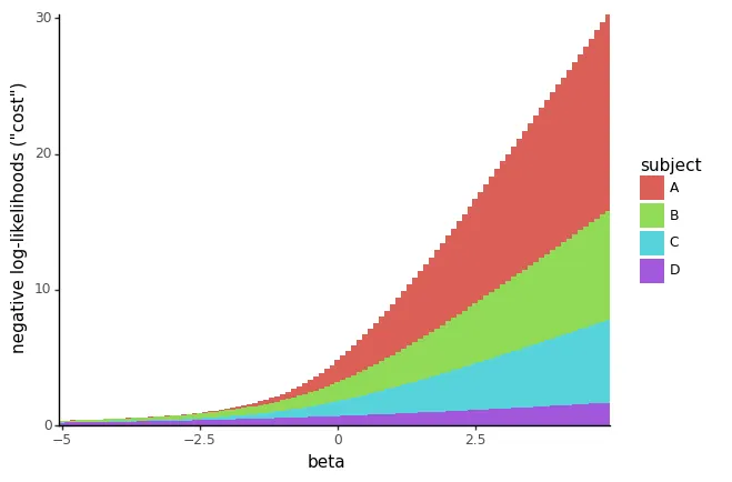
You possibly can see straight away that there isn’t a minimal worth of β any longer: if we use very giant unfavorable values of β, we find yourself with log-likelihood matches which can be near-perfect for all occasions.
Now, let’s dive into the maths behind this and try the chance of occasion A. We’ll dig into how the numerator and denominator change as we tweak β:

When β is excessive or a big optimistic quantity, the final time period within the denominator (with the biggest x of 1.2), representing the hazard of topic E, dominates your entire denominator and turns into exceedingly giant. So, the chance turns into small and approaches zero:

This ends in a giant unfavorable log-likelihood. The identical factor occurs for every particular person chance as a result of the final hazard of topic E, will all the time exceed any hazard within the numerator. Because of this, the unfavorable log-likelihood will increase for topics A to D. On this case, when we’ve got excessive β, it brings down all of the likelihoods, leading to poor matches for all occasions.
Now, when β is low or a giant unfavorable quantity, the primary time period within the denominator, representing the hazard of topic A, dominates because it has the bottom x worth. As the identical hazard of topic A additionally seems within the numerator, the chance L(A) will be arbitrarily near 1 by making β more and more unfavorable, thereby creating an virtually good match:

The identical deal goes for all the opposite particular person likelihoods: unfavorable βs now increase the likelihoods of all occasions on the identical time. Mainly, having a unfavorable β doesn’t include any downsides. On the identical time, sure particular person hazards improve (topics A and B with unfavorable x), some keep the identical (topic C with x = 0), and others lower (topic D with optimistic x). However bear in mind, what actually issues listed here are ratios of hazards. We will confirm this hand-waving math by plotting particular person hazards:
def plot_likelihoods(df, ylim=[-20, 20]):
betas = np.arange(ylim[0], ylim[1], 0.5)
topics = df.question("occasion == 1")['subject'].tolist()
likelihoods_per_subject = []
for topic in topics:
likelihoods = [
np.exp(log_likelihood(df, subject, beta))
for beta in betas
]
likelihoods_per_subject.append(
pd.DataFrame({
'beta': betas,
'chance': likelihoods,
'topic': [subject] * len(betas),
})
)
lik_df = pd.concat(likelihoods_per_subject)
return (
p9.ggplot(lik_df, p9.aes('beta', 'chance', colour='topic'))
+ p9.geom_line(measurement=2)
+ p9.theme_classic()
)    plot_likelihoods(perfect_df)

The way in which likelihoods are put collectively, as a ratio of a hazard to the sum of hazards of all topics nonetheless in danger, signifies that unfavorable β values make a good match for the chance of every topic whose occasion time rank is bigger than or equal to the predictor rank! As a aspect word, if x had an ideal unfavorable Spearman correlation with occasion occasions, issues could be flipped round: arbitrarily optimistic βs would give us arbitrarily good matches.

