
Introduction
Orthonormal vectors are a set of vectors which are each orthogonal (perpendicular) to one another and have a unit size (norm) of 1. In different phrases, the dot product of any two distinct vectors within the set is zero, and the dot product of a vector with itself is 1. Orthonormal vectors play an important function in machine studying, significantly within the context of dimensionality discount and have extraction. Strategies comparable to Principal Part Evaluation (PCA) depend on discovering orthonormal bases that may optimally signify the variance within the information, enabling environment friendly compression and noise discount.
Moreover, orthonormal vectors are utilized in numerous machine studying algorithms to simplify computations, enhance numerical stability, and facilitate the interpretation of outcomes. Their orthogonal nature ensures that the scale within the reworked area are impartial and uncorrelated, which is commonly a fascinating property in machine studying fashions.
Linear algebra, which offers with vectors and matrices, is likely one of the basic branches of arithmetic for machine studying. Vectors are sometimes used to signify information factors or options, whereas matrices are used to signify collections of information factors or units of options. In picture recognition duties, a picture might be represented as a vector of pixel values, and a set of photographs might be represented as a matrix the place every row corresponds to a picture vector.
By utilizing vectors to signify information, machine studying or deep studying algorithms can apply mathematical operations comparable to matrix multiplication and dot merchandise to govern and analyze the info. For instance, vector operations comparable to cosine similarity can be utilized to measure the similarity between two information factors or to mission high-dimensional information onto a lower-dimensional area for visualization or evaluation. By grouping related vectors collectively or predicting the worth of a goal variable based mostly on the values of different variables, these algorithms could make predictions or establish patterns within the information.
There are several types of vectors comparable to orthogonal vector, orthonormal vector, column vector, row vector, dimensional function vector, impartial vector, resultant function vector, and so on.
The distinction between a column vector and a row vector is primarily a matter of conference and notation. Typically, the selection of whether or not to make use of a column vector or a row vector depends upon the context and the precise software.
Dimensional function vector is a illustration of an object or entity that captures related details about its properties and traits in a multidimensional area. In different phrases, it’s a set of options or attributes that describe an object, and every function is assigned a worth in a numerical vector.
A vector is taken into account an impartial vector if no vector might be expressed as a linear mixture of these listed earlier than it within the set. impartial vector impartial vector.
Resultant function vector is a vector that summarizes or combines a number of function vectors right into a single vector that captures crucial info from the unique vectors. The method of mixing function vectors is known as function aggregation, and it’s usually utilized in machine studying and information evaluation functions the place a number of sources of data should be mixed to decide or prediction. Resultant function vectors might be helpful in lowering the dimensionality of information and in summarizing complicated info right into a extra manageable type. They’re extensively utilized in functions comparable to picture and speech recognition, pure language processing, and suggestion techniques.
Additionally Learn: What is a Sparse Matrix? How is it Used in Machine Learning?
Orthogonal and Orthonormal Vectors
Within the context of information evaluation and modeling, it may be helpful to rework the unique variables or enter variables into a brand new set of variables which are orthogonal or orthonormal. Explanatory variables might be regarded as the parts of the vector which are used to elucidate or predict a response variable and its parts might be regarded as quantitative variables.
Orthogonal and orthonormal vector algorithms play an essential in machine studying as a result of they allow environment friendly computations, simplify many mathematical operations, and may enhance the efficiency of many machine studying algorithms.
What are orthogonal vectors?
The phrase orthogonal comes from the Greek which means “right-angled”. An orthogonal vector is a vector that’s perpendicular to a different vector or set of vectors. In different phrases, the dot product of two orthogonal vectors is zero, which signifies that they don’t have any part in the identical path.
For instance, in two-dimensional area, the vector (1, 0) is orthogonal to the vector (0, 1), since their dot product is 10 + 01 = 0. Equally, in three-dimensional area, the vector (1, 0, 0) is orthogonal to each (0, 1, 0) and (0, 0, 1).
2D and 3D Orthogonal Vector
Orthogonal vectors are sometimes utilized in linear algebra, the place they’re used to assemble orthogonal bases for vector areas, which might simplify calculations and make them extra environment friendly. Linear mixtures of vectors are additionally used steadily in linear algebra, the place they can be utilized to signify any vector in a given area as a linear mixture of a set of foundation vectors.
It’s essential to notice that ordinary vector and orthogonal vector is commonly used interchangeably to confer with a vector that’s perpendicular to a different vector or floor, nevertheless there’s a delicate distinction between the 2 ideas. Regular vector is often used to explain a vector that’s perpendicular to a floor whereas orthogonal vector is extra basic and may confer with any two vectors which are perpendicular to one another.
In machine studying, linear mixtures of orthogonal vectors are utilized in numerous methods, comparable to in dimensionality discount strategies like Principal Part Evaluation (PCA). By utilizing linear mixtures of orthogonal vectors to signify the info, we will obtain a extra environment friendly and efficient illustration that captures crucial points of the info, whereas lowering noise and redundancy. This may enhance the efficiency of machine studying algorithms by lowering overfitting, enhancing generalization, and lowering computational complexity. In sample recognition, orthogonal vectors are utilized in numerous methods, comparable to in function extraction and classification algorithms.
Additionally Learn: Introduction to Vector Norms: L0, L1, L2, L-Infinity
Orthogonal matrices
An orthogonal matrix is a sq. matrix whose columns and rows are orthogonal to one another. Sq. matrix means the variety of rows and columns is identical. It’s a particular sort of matrix that makes use of transposes and inverses. A mirrored image matrix is a specific sort of orthogonal matrix that describes a mirrored image of a vector or a degree throughout a given line or airplane. A mirrored image matrix is symmetric, which means that it is the same as its transpose.
Geometrically, an orthogonal matrix preserves the size and angle between vectors. Which means that when an orthogonal matrix is utilized to a vector, the ensuing vector is rotated and/or mirrored in a manner that preserves its size and angle with respect to different vectors.
There are a number of fascinating properties of orthogonal matrices
- Its transpose is the same as its inverse of matrix. The inverse of matrix is a matrix that, when multiplied by the unique matrix, provides the identification matrix because the consequence.
- Product of an orthogonal matrix with its transpose provides an identification matrix. In different phrases, if A is an orthogonal matrix, then A^T * A = A * A^T = I, the place I is the identification matrix.
- The transpose of an orthogonal matrix can also be at all times orthogonal
- The most important eigenvalue of an orthogonal matrix is at all times 1 or -1, as a result of the product of the eigenvalues of an orthogonal matrix is the same as the determinant, which for an orthogonal matrix is both 1 or -1.
Orthogonal matrices and matrix norms are an essential idea in linear algebra and matrix factorization. Matrix norm are used to measure the scale of a matrix or a vector, which might be useful in regularization and avoiding overfitting. Matrix factorization is a way in linear algebra that includes decomposing a matrix right into a product of less complicated matrices. The objective of matrix factorization is commonly to signify the unique matrix in a extra compact type that’s simpler to investigate or manipulate. Different matrix factorization strategies, comparable to QR factorization and Cholesky decomposition, additionally contain discovering units of orthogonal vectors that can be utilized to simplify the matrix illustration. They’re utilized in a wide range of functions, together with laptop graphics, physics, engineering, and cryptography.
It’s also fascinating to discover the relation between orthogonal matrix and different forms of matrices related to machine studying comparable to unitary matrix, diagonal matrix, triangular matrix, symmetric matrix and rating matrix.
Unitary matrix
A unitary matrix, is a fancy sq. matrix the place the columns are all unitary vectors, which means that they’re orthogonal to one another and have a size of 1 within the complicated sense. In different phrases, if U is a unitary matrix, then U^H * U = U * U^H = I, the place U^H is the Hermitian transpose of U. The connection between orthogonal matrices and unitary matrices is that each orthogonal matrix is a real-valued unitary matrix. Which means that if A is an orthogonal matrix, then it is usually a unitary matrix when seen as a fancy matrix with zeros within the imaginary half. Conversely, each unitary matrix with actual entries is an orthogonal matrix.In deep studying, unitary matrices are utilized in numerous contexts, comparable to within the design of neural networks and within the computation of quantum-inspired algorithms.
Unitary matrices are essential in lots of areas of machine studying, comparable to:
- Singular Worth Decomposition (SVD): In Singular Worth Decomposition, a matrix is factorized into three matrices, considered one of which is a unitary matrix. This unitary matrix represents the rotation or transformation of the unique information.
- Sign processing: Unitary matrices can be utilized for Fourier evaluation, which is a way utilized in sign processing to decompose a sign into its frequency parts.
Diagonal matrix
A diagonal matrix is a sq. matrix the place all of the off-diagonal parts are zero, and the diagonal parts might be any worth. An instance of a diagonal matrix is the matrix of eigenvalues in eigendecomposition. The connection between orthogonal matrix and diagonal matrix is that each orthogonal matrix might be decomposed right into a product of a diagonal matrix and an orthogonal matrix that’s its transpose. This decomposition is named the singular worth decomposition (SVD), and it may be written as follows:
A = U * D * V^T
The place A is the orthogonal matrix, U and V are orthogonal matrices, and D is a diagonal matrix. The columns of U and V are the left and proper singular vectors of A, respectively, and the diagonal parts of D are the singular values of A. The Singular Worth Decomposition is a strong device in linear algebra and machine studying, as it may be used for numerous duties comparable to dimensionality discount, matrix compression, and matrix inversion.
Diagonal matrices are utilized in numerous areas of machine studying, comparable to:
- Principal Part Evaluation (PCA): Linear mixtures of orthogonal vectors are sometimes used as a manner of representing information in a lower-dimensional area, a way referred to as principal part evaluation (PCA). The important thing ideas in PCA embrace orthogonal vectors, customary deviation, squared error, correlation matrix, eigenvalues and eigenvectors. The unique variables are reworked right into a set of orthonormal variables and the covariance matrix is diagonalized to seek out the principal parts. This diagonalization is completed by discovering the eigenvectors and eigenvalues of the covariance matrix, which is commonly a symmetric positive-definite matrix.
- Regularization: In regularization, diagonal matrices are added to the unique matrix to stop overfitting. These diagonal matrices are sometimes called “penalty” or “shrinkage” phrases.
- Transformation: Diagonal matrices can be utilized to rework a dataset. For instance, in sign processing, diagonal matrices can be utilized to signify filters.
Triangular matrix
A triangular matrix is a sq. matrix the place all the weather above or under the primary diagonal are zero. The principle diagonal is the road that runs from the top-left nook of the matrix to the bottom-right nook. Each orthogonal matrix might be decomposed right into a product of a triangular matrix and an orthogonal matrix: Any sq. matrix might be decomposed right into a product of a decrease triangular matrix and an higher triangular matrix. Within the case of an orthogonal matrix, we will decompose it right into a product of a decrease triangular matrix and an orthogonal matrix through the use of the Gram-Schmidt course of. This decomposition is known as QR factorization, the place Q is an orthogonal matrix and R is an higher triangular matrix.
These relationships between orthogonal matrices and triangular matrices are essential in lots of areas of arithmetic and engineering, together with linear regression, sign processing, and numerical linear algebra.
Symmetric matrix
A symmetric matrix is a sq. matrix the place the weather above and under the diagonal are mirror photographs of one another. In different phrases, A[i,j] = A[j,i] for all i and j. A symmetric matrix is at all times diagonalizable, which signifies that it may be decomposed right into a product of its eigenvectors and eigenvalues. The connection between orthogonal and symmetric matrices is that if A is a symmetric matrix, then its eigenvectors are orthogonal to one another. Moreover, the eigenvectors of a symmetric matrix might be chosen to be orthonormal, which signifies that they’re orthogonal to one another and have a size of 1. In different phrases, the eigenvectors of a symmetric matrix type an orthonormal foundation. This connection between orthogonal and symmetric matrices is helpful in lots of areas of deep studying the place symmetric matrices come up steadily.
This makes them significantly helpful in lots of functions, comparable to principal part evaluation and spectral clustering.
Rating matrix
A rating matrix is a matrix that’s used to assign scores or penalties to pairs of sequences in a sequence alignment. Rating matrices are utilized in bioinformatics and computational biology to attain sequence alignments based mostly on their similarity. Orthogonal matrices can be utilized in sure functions associated to sequence alignment and rating matrices. For instance, in some strategies for calculating the optimum sequence alignment rating utilizing dynamic programming, the algorithm includes calculating the rating matrix recursively. The matrix multiplication step concerned on this algorithm might be seen as equal to remodeling one rating matrix into one other utilizing an orthogonal matrix.
Additionally Learn: PCA-Whitening vs ZCA Whitening: What is the Difference?
What are orthonormal vectors?
An orthonormal vector is a vector that has a magnitude (size) of 1 and is perpendicular (orthogonal) to all different vectors in a given set of vectors. In different phrases, a set of orthonormal vectors types an orthogonal foundation for the vector area wherein they reside. The time period “ortho” comes from the Greek phrase for “perpendicular,” whereas “regular” is used to point that the vectors have a size of 1, which can also be known as being normalized. It’s also referred to as an orthogonal unit vector.
A set of vectors {v1, v2, …, vn} is orthonormal if:
- Every vector vi is a unit vector, which means that ||vi|| = 1.
- Every vector vi is orthogonal to each different vector vj, the place i and j are distinct indices.
In linear algebra, orthonormal vectors are sometimes used to simplify calculations and signify geometric ideas. They’re generally utilized in functions comparable to laptop graphics, sign processing, and quantum mechanics, amongst others. In sample recognition, orthonormal vectors are utilized in numerous methods, comparable to in dimensionality discount, function extraction, and classification algorithms. Some algorithms that make use of orthogonal vectors embrace Singular Worth Decomposition (SVD). SVD is a well-liked technique used for dimensionality discount and Haar Remodel, a way used for compressing digital photographs.
Visualization of Orthogonal Vectors
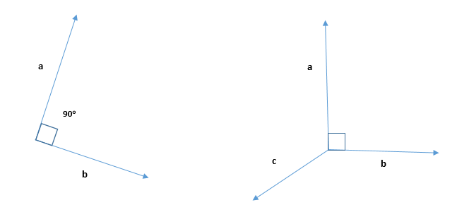
To visualise orthogonal vectors, we will use a 2D or 3D coordinate system.
In 2D, we will think about two vectors which are perpendicular to one another, with one vector pointing horizontally (alongside the x-axis) and the opposite pointing vertically (alongside the y-axis). The 2 vectors type a proper angle on the origin of the coordinate system.
Python code
#matplotib and numpy import
import matplotlib.pyplot as plt
import numpy as np

fig = plt.determine(figsize=(4, 4))
ax = fig.add_subplot(111)

ax.grid(alpha=0.4)
ax.set(xlim=(-3, 3), ylim=(-3, 3))

#numpy import array
v1 = np.array([1, 2])
v2 = np.array([2, -1])

# Plot the orthogonal vectors
ax.annotate('', xy=v1, xytext=(0, 0), arrowprops=dict(facecolor='b'))
ax.annotate('', xy=v2, xytext=(0, 0), arrowprops=dict(facecolor='g'))

plt.present()
In 3D, we will think about three vectors which are mutually orthogonal to one another. We will visualize this by drawing three axes: the x-axis, y-axis, and z-axis. The three axes type a right-handed coordinate system. The vector alongside the x-axis is orthogonal to each the y-axis and the z-axis, the vector alongside the y-axis is orthogonal to each the x-axis and the z-axis, and the vector alongside the z-axis is orthogonal to each the x-axis and the y-axis.
Python code
#matplotib and numpy import
import matplotlib.pyplot as plt
import numpy as np

fig = plt.determine(figsize=(7,7))
ax = fig.add_subplot(111, projection="3d")

#Outline the orthogonal vectors
#numpy import array
v1 = np.array([0, 0, -1])
v2 = np.array([1, 1, 0])
v3 = np.array([-1, 1, 0])

# Plot the orthogonal vectors
ax.quiver(0,0,0, v1[0], v1[1], v1[2], colour='r', lw=3, arrow_length_ratio=0.2)
ax.quiver(0,0,0, v2[0], v2[1], v2[2], colour='g', lw=3, arrow_length_ratio=0.2)
ax.quiver(0,0,0, v3[0], v3[1], v3[2], colour='b', lw=3, arrow_length_ratio=0.2)

ax.set_xlim([-1, 1]), ax.set_ylim([-1, 1]), ax.set_zlim([-1, 1])
ax.set_xlabel('X axis'), ax.set_ylabel('Y axis'), ax.set_zlabel('Z axis')
plt.present()
We will additionally use geometric shapes to visualise orthogonal vectors. For instance, in 2D, we will draw a rectangle with sides parallel to the x-axis and y-axis. The edges of the rectangle signify the orthogonal vectors. Equally, in 3D, we will draw an oblong prism with sides parallel to the x-axis, y-axis, and z-axis. The sides of the oblong prism signify the orthogonal vectors.
Additionally Learn: How to Use Linear Regression in Machine Learning.
Orthogonal Vectors Histogram (OVH)
An orthogonal vector histogram is a solution to signify a set of vectors in a high-dimensional area. The fundamental thought behind an orthogonal vector histogram is to partition the area right into a set of orthogonal subspaces after which rely the variety of vectors that lie inside every subspace.
To create an orthogonal vector histogram, we first select a set of orthogonal foundation vectors that span the area. For instance, in 3D area, we would select the three unit vectors alongside the x, y, and z axes. Subsequent, we divide every axis right into a set of bins or intervals, and we rely the variety of unit vectors that fall into every bin. For instance, if we divide every axis into 10 bins, we’d rely the variety of vectors that fall into every of the ten x-bins, every of the ten y-bins, and every of the ten z-bins.Lastly, we signify the counts in a histogram or bar chart, with every bin or interval alongside every axis equivalent to a bar within the chart.The ensuing histogram supplies a visualization of the distribution of vectors within the high-dimensional area, with every bar representing the variety of vectors that fall into a specific area of the area. The usage of orthogonal subspaces and bins permits us to signify complicated distributions in a easy and intuitive manner.
Orthogonal vector histograms are a strong approach for sample recognition and classification. In sample recognition, the objective is to establish and categorize objects based mostly on their underlying options, comparable to form, colour, texture, or orientation. Orthogonal vector histograms can be utilized to extract and signify these options in a high-dimensional area, permitting us to check and classify objects based mostly on their similarity on this area. OVH can be utilized in picture classification duties as a solution to signify picture options in a high-dimensional area. On this context, every picture might be represented as a set of vectors, the place every vector corresponds to a specific function of the picture. To create an orthogonal vector histogram for a picture, we first extract a set of options from the picture utilizing strategies comparable to edge detection, texture evaluation, or colour histogramming. Every function is then represented as a vector in a high-dimensional area, with every dimension equivalent to a specific side of the function (e.g., orientation, texture, colour). We will then create an orthogonal vector histogram by dividing the high-dimensional area right into a set of orthogonal subspaces and counting the variety of function vectors that fall into every subspace. The ensuing histogram supplies a compact illustration of the picture options, capturing the important info wanted for picture classification.
Implementation particulars
In laptop imaginative and prescient, labeling photographs into semantic classes is a difficult drawback to unravel. Picture classification is a difficult job due to a number of traits related to the picture comparable to illumination, litter, partial occlusion and others. Bag of visible phrases (BOVW) is a extensively used machine studying mannequin in picture classification. Its idea is customized from NLP’s bag of phrases (BOW) the place we rely the variety of instances every phrase seems in a doc, use the frequency of the phrases to find out the key phrases and make a frequency histogram. It doesn’t retain the order of the phrases. In BoVW mannequin, the native options are quantized and 2-D picture area is represented within the type of order-less histogram of visible phrases however the picture classification efficiency suffers as a result of order-less illustration of picture.
A analysis revealed within the doi journal offered a novel solution to mannequin world relative spatial orientation of visible phrases in a rotation invariant method which demonstrated outstanding acquire within the classification accuracy over the state-of-the-art strategies. 4 picture benchmarks had been used to validate the method.
The determine and the main points that comply with describes the method:
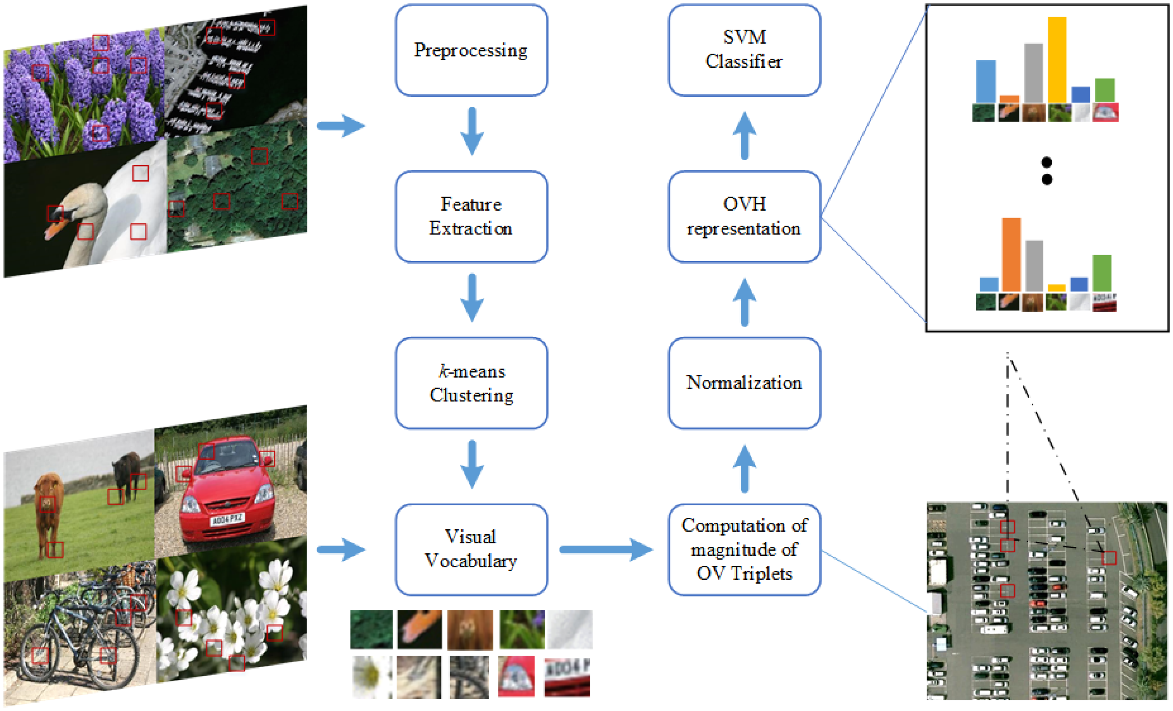
Block diagram of proposed analysis based mostly on OVH
Supply: doi
- Pre-processing step – giant photographs are resized to a regular dimension of 480 × 480 pixels.
- Characteristic extraction – all photographs are transformed to grey scale.
- Ok-means clustering – is used to generate the visible vocabulary. Since Ok-means is unsupervised, the experiment is repeated a number of instances with random number of coaching and check photographs.
- OV triplets – A threshold and a random choice is used to restrict the variety of phrases of the identical sort used for the creating triplet mixtures.
- OVH illustration – A 5-bin OVH illustration for the outcomes is offered.
- Classification – Assist Vector Machines (SVM) is used for classification. Kernel technique is used to generate non-linear choice boundaries. The ensuing histogram is normalized and SVM Hellinger Kernel is utilized due to its low compute price. SVM Hellinger kernel can explicitly compute the options map as a substitute of computing the kernel values and the classifier stays linear. A ten-fold cross validation is utilized on the coaching dataset to find out the optimum worth. The one-against-one method is utilized. On this method, a binary classifier is skilled for every potential pair of lessons within the dataset. One benefit of the one-against-one method is that it may be extra computationally environment friendly than different approaches, particularly when there are various lessons.
The 4 customary picture benchmarks included the next datasets:
- 15-scene picture dataset – comprised a variety of indoor and out of doors class photographs together with private images, the Web and COREL collections. The dataset included 4485 photographs with a median picture dimension 300 × 250 pixels.
- MSRC-v2 picture dataset – consisted of 591 photographs categorized into 23 classes. The objects exhibited intra-class variation in form and dimension, along with partial occlusion.
- UC Merced land-use (UCM) picture dataset – comprised 21 land-use lessons from the US Geological Survey (USGS) Nationwide map. Every class contained 100 photographs of dimension 256 × 256 pixels offering giant geographical scale.
- 19-class satellite tv for pc scene picture dataset – comprised 19 high-resolution satellite tv for pc scene classes with a deal with This dataset targeted on photographs with a big geographical scale and contained a minimum of 50 photographs/class, dimension 600 × 600 pixels.
The outcomes efficiently included relative world spatial info into the BoVW mannequin. The proposed method outperformed different concurrent native and world histogram based mostly strategies and offered a aggressive efficiency.
Additionally Learn: What Are Support Vector Machines (SVM) In Machine Learning
Conclusion and future instructions
Orthogonal vectors and histograms are a strong device in sample recognition, as they allow us to establish probably the most informative options, separate the completely different lessons, and cluster the info in an environment friendly and efficient manner. General, orthogonal vector histograms present a strong and versatile solution to signify picture options, and can be utilized in a variety of picture classification duties, together with object recognition, scene classification, and face recognition.

References
Picture classification by addition of spatial info based mostly on histograms of orthogonal vectors https://doi.org/10.1371/journal.pone.0198175. Accessed 30 Mar. 2023
Vedaldi A, Zisserman A. Sparse kernel approximations for environment friendly classification and detection. In: Pc Imaginative and prescient and Sample Recognition (CVPR), 2012 IEEE Convention on. IEEE; 2012. p. 2320–2327. Accessed 30 Mar. 2023
Fatih Karabiber, “Orthogonal and Orthonormal Vectors”, https://www.learndatasci.com/glossary/orthogonal-and-orthonormal-vectors. Accessed 1 Apr. 2023
Ali N, Bajwa KB, Sablatnig R, Chatzichristofis SA, Iqbal Z, Rashid M, et al. “A Novel Picture Retrieval Based mostly on Visible Phrases Integration of SIFT and SURF”, https://journals.plos.org/plosone/article?id=10.1371/journal.pone.0157428. Accessed 30 Mar. 2023
Bethea Davida, “Bag of Visible Phrases in a Nutshell”, https://towardsdatascience.com/bag-of-visual-words-in-a-nutshell-9ceea97ce0fb. Accessed 1 Apr. 2023
Chatzichristofis SA, Iakovidou C, Boutalis Y, Marques O. Co. vi. wo.: colour visible phrases based mostly on non-predefined dimension codebooks. IEEE transactions on cybernetics. 2013;43(1):192–205. pmid:22773049. Accessed 2 Apr. 2023

