
Latest years have proven wonderful development in deep studying neural networks (DNNs). This development will be seen in additional correct fashions and even opening new potentialities with generative AI: massive language fashions (LLMs) that synthesize pure language, text-to-image mills, and extra. These elevated capabilities of DNNs include the price of having large fashions that require vital computational sources so as to be educated. Distributed coaching addresses this drawback with two methods: information parallelism and mannequin parallelism. Information parallelism is used to scale the coaching course of over a number of nodes and employees, and mannequin parallelism splits a mannequin and matches them over the designated infrastructure. Amazon SageMaker distributed training jobs allow you with one click on (or one API name) to arrange a distributed compute cluster, prepare a mannequin, save the consequence to Amazon Simple Storage Service (Amazon S3), and shut down the cluster when full. Moreover, SageMaker has constantly innovated within the distributed coaching area by launching options like heterogeneous clusters and distributed coaching libraries for data parallelism and model parallelism.
Environment friendly coaching on a distributed surroundings requires adjusting hyperparameters. A typical instance of excellent follow when coaching on a number of GPUs is to multiply batch (or mini-batch) measurement by the GPU quantity so as to hold the identical batch measurement per GPU. Nevertheless, adjusting hyperparameters usually impacts mannequin convergence. Due to this fact, distributed coaching must stability three components: distribution, hyperparameters, and mannequin accuracy.
On this publish, we discover the impact of distributed coaching on convergence and use Amazon SageMaker Automatic Model Tuning to fine-tune mannequin hyperparameters for distributed coaching utilizing information parallelism.
The supply code talked about on this publish will be discovered on the GitHub repository (an m5.xlarge occasion is really useful).
Scale out coaching from a single to distributed surroundings
Information parallelism is a strategy to scale the coaching course of to a number of compute sources and obtain quicker coaching time. With information parallelism, information is partitioned among the many compute nodes, and every node computes the gradients primarily based on their partition and updates the mannequin. These updates will be executed utilizing one or a number of parameter servers in an asynchronous, one-to-many, or all-to-all trend. One other method will be to make use of an AllReduce algorithm. For instance, within the ring-allreduce algorithm, every node communicates with solely two of its neighboring nodes, thereby decreasing the general information transfers. To study extra about parameter servers and ring-allreduce, see Launching TensorFlow distributed training easily with Horovod or Parameter Servers in Amazon SageMaker. Almost about information partitioning, if there are n compute nodes, then every node ought to get a subset of the info, roughly 1/n in measurement.
To show the impact of scaling out coaching on mannequin convergence, we run two easy experiments:
Every mannequin coaching ran twice: on a single occasion and distributed over a number of situations. For the DNN distributed coaching, so as to totally make the most of the distributed processors, we multiplied the mini-batch measurement by the variety of situations (4). The next desk summarizes the setup and outcomes.
| Drawback sort | Picture classification | Binary classification | ||
| Mannequin | DNN | XGBoost | ||
| Occasion | ml.c4.xlarge | ml.m5.2xlarge | ||
| Information set |
(Labeled pictures) |
Direct Marketing (tabular, numeric and vectorized classes) |
||
| Validation metric | Accuracy | AUC | ||
| Epocs/Rounds | 20 | 150 | ||
| Variety of Situations | 1 | 4 | 1 | 3 |
| Distribution sort | N/A | Parameter server | N/A | AllReduce |
| Coaching time (minutes) | 8 | 3 | 3 | 1 |
| Remaining Validation rating | 0.97 | 0.11 | 0.78 | 0.63 |
For each fashions, the coaching time was decreased virtually linearly by the distribution issue. Nevertheless, mannequin convergence suffered a big drop. This conduct is constant for the 2 completely different fashions, the completely different compute situations, the completely different distribution strategies, and completely different information varieties. So, why did distributing the coaching course of have an effect on mannequin accuracy?
There are a selection of theories that attempt to clarify this impact:
- When tensor updates are massive in measurement, site visitors between employees and the parameter server can get congested. Due to this fact, asynchronous parameter servers will endure considerably worse convergence on account of delays in weights updates [1].
- Growing batch measurement can result in over-fitting and poor generalization, thereby decreasing the validation accuracy [2].
- When asynchronously updating mannequin parameters, some DNNs won’t be utilizing the latest up to date mannequin weights; subsequently, they are going to be calculating gradients primarily based on weights which can be just a few iterations behind. This results in weight staleness [3] and will be brought on by a lot of causes.
- Some hyperparameters are mannequin or optimizer particular. For instance, the XGBoost official documentation says that the
actualworth for thetree_modehyperparameter doesn’t assist distributed coaching as a result of XGBoost employs row splitting information distribution whereas theactualtree technique works on a sorted column format. - Some researchers proposed that configuring a bigger mini-batch could result in gradients with much less stochasticity. This may occur when the loss perform incorporates native minima and saddle factors and no change is made to step measurement, to optimization getting caught in such native minima or saddle level [4].
Optimize for distributed coaching
Hyperparameter optimization (HPO) is the method of looking and deciding on a set of hyperparameters which can be optimum for a studying algorithm. SageMaker Computerized Mannequin Tuning (AMT) offers HPO as a managed service by working a number of coaching jobs on the offered dataset. SageMaker AMT searches the ranges of hyperparameters that you just specify and returns one of the best values, as measured by a metric that you just select. You need to use SageMaker AMT with the built-in algorithms or use your customized algorithms and containers.
Nevertheless, optimizing for distributed coaching differs from widespread HPO as a result of as an alternative of launching a single occasion per coaching job, every job really launches a cluster of situations. This implies a higher affect on value (particularly in case you contemplate expensive GPU-accelerated situations, that are typical for DNN). Along with AMT limits, you might presumably hit SageMaker account limits for concurrent variety of coaching situations. Lastly, launching clusters can introduce operational overhead on account of longer beginning time. SageMaker AMT has particular options to handle these points. Hyperband with early stopping ensures that well-performing hyperparameters configurations are fine-tuned and people who underperform are robotically stopped. This permits environment friendly use of coaching time and reduces pointless prices. Additionally, SageMaker AMT totally helps the usage of Amazon EC2 Spot Situations, which might optimize the cost of training up to 90% over on-demand situations. Almost about lengthy begin occasions, SageMaker AMT robotically reuses coaching situations inside every tuning job, thereby decreasing the typical startup time of every training job by 20 times. Moreover, you must observe AMT best practices, resembling selecting the related hyperparameters, their applicable ranges and scales, and one of the best variety of concurrent coaching jobs, and setting a random seed to breed outcomes.
Within the subsequent part, we see these options in motion as we configure, run, and analyze an AMT job utilizing the XGBoost instance we mentioned earlier.
Configure, run, and analyze a tuning job
As talked about earlier, the supply code will be discovered on the GitHub repo. In Steps 1–5, we obtain and put together the info, create the xgb3 estimator (the distributed XGBoost estimator is about to make use of three situations), run the coaching jobs, and observe the outcomes. On this part, we describe arrange the tuning job for that estimator, assuming you already went by means of Steps 1–5.
A tuning job computes optimum hyperparameters for the coaching jobs it launches by utilizing a metric to guage efficiency. You’ll be able to configure your own metric, which SageMaker will parse primarily based on regex you configure and emit to stdout, or use the metrics of SageMaker built-in algorithms. On this instance, we use the built-in XGBoost objective metric, so we don’t have to configure a regex. To optimize for mannequin convergence, we optimize primarily based on the validation AUC metric:
We tune seven hyperparameters:
- num_round – Variety of rounds for enhancing through the coaching.
- eta – Step measurement shrinkage utilized in updates to forestall overfitting.
- alpha – L1 regularization time period on weights.
- min_child_weight – Minimal sum of occasion weight (hessian) wanted in a baby. If the tree partition step ends in a leaf node with the sum of occasion weight lower than
min_child_weight, the constructing course of offers up additional partitioning. - max_depth – Most depth of a tree.
- colsample_bylevel – Subsample ratio of columns for every break up, in every degree. This subsampling takes place as soon as for each new depth degree reached in a tree.
- colsample_bytree – Subsample ratio of columns when developing every tree. For each tree constructed, the subsampling happens as soon as.
To study extra about XGBoost hyperparameters, see XGBoost Hyperparameters. The next code reveals the seven hyperparameters and their ranges:
Subsequent, we offer the configuration for the Hyperband strategy and the tuner object configuration utilizing the SageMaker SDK. HyperbandStrategyConfig can use two parameters: max_resource (non-compulsory) for the utmost variety of iterations for use for a coaching job to realize the target, and min_resource – the minimal variety of iterations for use by a coaching job earlier than stopping the coaching. We use HyperbandStrategyConfig to configure StrategyConfig, which is later utilized by the tuning job definition. See the next code:
Now we create a HyperparameterTuner object, to which we cross the next data:
- The XGBoost estimator, set to run with three situations
- The target metric title and definition
- Our hyperparameter ranges
- Tuning useful resource configurations resembling variety of coaching jobs to run in complete and what number of coaching jobs will be run in parallel
- Hyperband settings (the technique and configuration we configured within the final step)
- Early stopping (
early_stopping_type) set toOff
Why can we set early stopping to Off? Coaching jobs will be stopped early when they’re unlikely to enhance the target metric of the hyperparameter tuning job. This can assist scale back compute time and keep away from overfitting your mannequin. Nevertheless, Hyperband makes use of a sophisticated built-in mechanism to use early stopping. Due to this fact, the parameter early_stopping_type have to be set to Off when utilizing the Hyperband inside early stopping function. See the next code:
Lastly, we begin the automated mannequin tuning job by calling the fit technique. If you wish to launch the job in an asynchronous trend, set wait to False. See the next code:
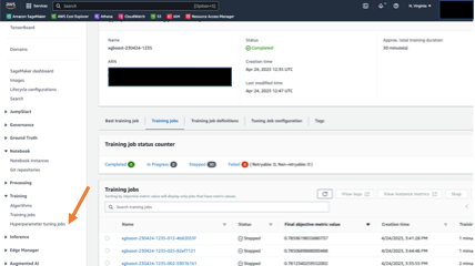
You’ll be able to observe the job progress and abstract on the SageMaker console. Within the navigation pane, below Coaching, select Hyperparameter tuning jobs, then select the related tuning job. The next screenshot reveals the tuning job with particulars on the coaching jobs’ standing and efficiency.
When the tuning job is full, we will evaluate the outcomes. Within the pocket book instance, we present extract outcomes utilizing the SageMaker SDK. First, we look at how the tuning job elevated mannequin convergence. You’ll be able to connect the HyperparameterTuner object utilizing the job title and name the describe technique. The tactic returns a dictionary containing tuning job metadata and outcomes.
Within the following code, we retrieve the worth of the best-performing coaching job, as measured by our goal metric (validation AUC):
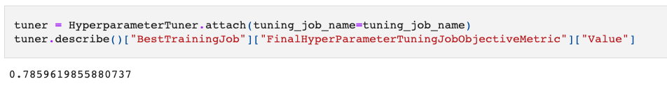
The result’s 0.78 in AUC on the validation set. That’s a big enchancment over the preliminary 0.63!
Subsequent, let’s see how briskly our coaching job ran. For that, we use the HyperparameterTuningJobAnalytics technique within the SDK to fetch outcomes in regards to the tuning job, and browse right into a Pandas information body for evaluation and visualization:
Let’s see the typical time a coaching job took with Hyperband technique:

The typical time took roughly 1 minute. That is in line with the Hyperband technique mechanism that stops underperforming coaching jobs early. When it comes to value, the tuning job charged us for a complete of half-hour of coaching time. With out Hyperband early stopping, the overall billable coaching period was anticipated to be 90 minutes (30 jobs * 1 minutes per job * 3 situations per job). That’s thrice higher in value financial savings! Lastly, we see that the tuning job ran 30 coaching jobs and took a complete of 12 minutes. That’s virtually 50% much less of the anticipated time (30 jobs/4 jobs in parallel * 3 minutes per job).
Conclusion
On this publish, we described some noticed convergence points when coaching fashions with distributed environments. We noticed that SageMaker AMT utilizing Hyperband addressed the primary considerations that optimizing information parallel distributed coaching launched: convergence (which improved by greater than 10%), operational effectivity (the tuning job took 50% much less time than a sequential, non-optimized job would have taken) and cost-efficiency (30 vs. the 90 billable minutes of coaching job time). The next desk summarizes our outcomes:
| Enchancment Metric | No Tuning/Naive Mannequin Tuning Implementation | SageMaker Hyperband Computerized Mannequin Tuning | Measured Enchancment |
| Mannequin High quality (Measured by validation AUC) |
0.63 | 0.78 | 15% |
| Price (Measured by billable coaching minutes) |
90 | 30 | 66% |
| Operational effectivity (Measured by complete working time) |
24 | 12 | 50% |
To be able to fine-tune almost about scaling (cluster measurement), you may repeat the tuning job with a number of cluster configurations and examine the outcomes to search out the optimum hyperparameters that fulfill velocity and mannequin accuracy.
We included the steps to realize this within the final part of the notebook.
References
[1] Lian, Xiangru, et al. “Asynchronous decentralized parallel stochastic gradient descent.” Worldwide Convention on Machine Studying. PMLR, 2018.
[2] Keskar, Nitish Shirish, et al. “On large-batch coaching for deep studying: Generalization hole and sharp minima.” arXiv preprint arXiv:1609.04836 (2016).
[3] Dai, Wei, et al. “Towards understanding the affect of staleness in distributed machine studying.” arXiv preprint arXiv:1810.03264 (2018).
[4] Dauphin, Yann N., et al. “Figuring out and attacking the saddle level drawback in high-dimensional non-convex optimization.” Advances in neural data processing methods 27 (2014).
Concerning the Writer
 Uri Rosenberg is the AI & ML Specialist Technical Supervisor for Europe, Center East, and Africa. Primarily based out of Israel, Uri works to empower enterprise clients to design, construct, and function ML workloads at scale. In his spare time, he enjoys biking, climbing, and complaining about information preparation.

