On this part, we’ll attempt to perceive if there’s a data-informed worthwhile strategy to ship the present, by focusing on particular prospects. Specifically, we’ll evaluate completely different focusing on insurance policies with the target of accelerating income.
All through this part, we’ll want some algorithms to both predict income, or churn, or the likelihood of receiving the present. We use gradient-boosted tree fashions from the lightgbm library. We use the identical fashions for all insurance policies in order that we can’t attribute variations in efficiency to prediction accuracy.
from lightgbm import LGBMClassifier, LGBMRegressor
To consider every coverage denoted with τ, we evaluate its income with the coverage Π⁽¹⁾, with its income with out the coverage Π⁽⁰⁾, over each single particular person, in a separate validation dataset. Notice that that is normally not doable since, for every buyer, we solely observe one of many two potential outcomes, with or with out the present. Nevertheless, since we’re working with artificial knowledge, we will do oracle analysis. If you wish to know extra about the way to consider uplift fashions with actual knowledge, I like to recommend my introductory article.
To start with, let’s outline income Π as the web income R when the shopper doesn’t churn C.

Subsequently, the general impact on income for handled people is given by the distinction between the income when handled Π⁽¹⁾ minus the income when not handled Π⁽⁰⁾.

The impact for untreated people is zero.
def evaluate_policy(coverage):
knowledge = dgp.generate_data(seed_data=4, seed_assignment=5, keep_po=True)
knowledge['profits'] = (1 - knowledge.churn) * knowledge.income
baseline = (1-data.churn_c) * knowledge.revenue_c
impact = coverage(knowledge) * (1-data.churn_t) * (knowledge.revenue_t-cost) + (1-policy(knowledge)) * (1-data.churn_c) * knowledge.revenue_c
return np.sum(impact - baseline)
1. Goal Churning Prospects
A primary coverage might be to only goal churning prospects. Let’s say we ship the present solely to prospects with above-average predicted churn.
model_churn = LGBMClassifier().match(X=df[X], y=df['churn'])policy_churn = lambda df : (model_churn.predict_proba(df[X])[:,1] > df.churn.imply())
evaluate_policy(policy_churn)
-5497.46
The coverage will not be worthwhile and would result in an combination loss of greater than 5000$.
You may assume that the issue is the arbitrary threshold, however this isn’t the case. Beneath I plot the mixture impact for all doable coverage thresholds.
x = np.linspace(0, 1, 100)
y = [evaluate_policy(lambda df : (model_churn.predict_proba(df[X])[:,1] > p)) for pin x]fig, ax = plt.subplots(figsize=(10, 3))
sns.lineplot(x=x, y=y).set(xlabel='Churn Coverage Threshold', title='Mixture Impact');
ax.axhline(y=0, c='ok', lw=3, ls='--');
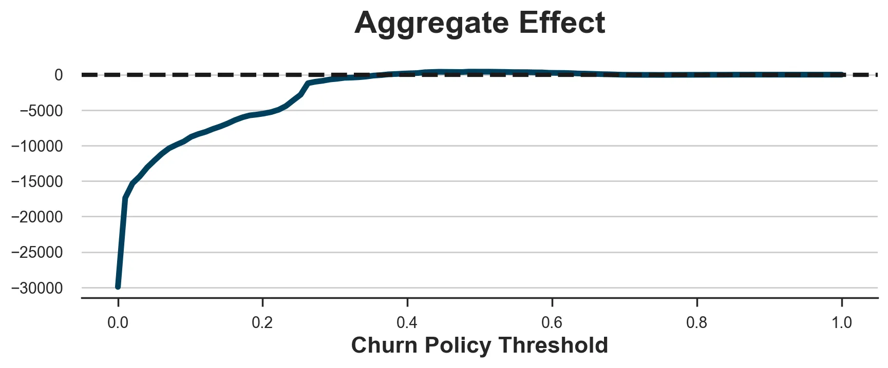
As we will see, irrespective of the brink, it’s principally unimaginable to make any revenue.
The issue is that the truth that a buyer is more likely to churn doesn’t indicate that the present can have any affect on their churn likelihood. The 2 measures are usually not utterly unrelated (e.g. we can’t lower the churning likelihood of consumers which have a 0% likelihood of churning), however they don’t seem to be the identical factor.
2. Goal income prospects
Let’s now strive a distinct coverage: we ship the present solely to high-revenue prospects. For instance, we would ship the present solely to the highest 10% of consumers by income. The thought is that if the coverage certainly decreases churn, these are the shoppers for whom reducing churn is extra worthwhile.
model_revenue = LGBMRegressor().match(X=df[X], y=df['revenue'])policy_revenue = lambda df : (model_revenue.predict(df[X]) > np.quantile(df.income, 0.9))
evaluate_policy(policy_revenue)
-4730.82
The coverage is once more unprofitable, resulting in substantial losses. As earlier than, this isn’t an issue of choosing the brink, as we will see within the plot beneath. One of the best we will do is ready a threshold so excessive that we don’t deal with anybody, and we make zero income.
x = np.linspace(0, 100, 100)
y = [evaluate_policy(lambda df : (model_revenue.predict(df[X]) > c)) for c in x]fig, ax = plt.subplots(figsize=(10, 3))
sns.lineplot(x=x, y=y).set(xlabel='Income Coverage Threshold', title='Mixture Impact');
ax.axhline(y=0, c='ok', lw=3, ls='--');
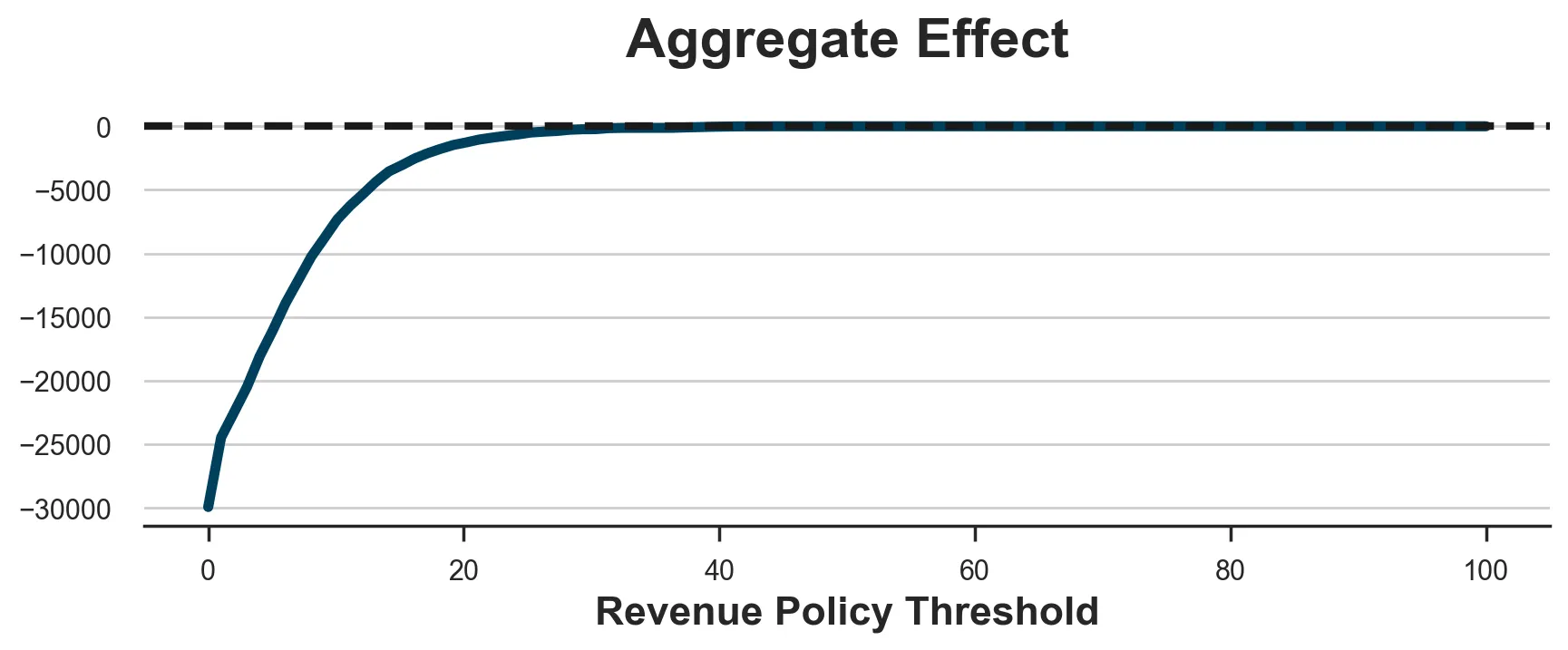
The issue is that, in our setting, the churn likelihood of high-revenue prospects doesn’t lower sufficient to make the present worthwhile. That is additionally partially as a result of reality, typically noticed in actuality, that high-revenue prospects are additionally the least more likely to churn, to start with.
Let’s now take into account a extra related set of insurance policies: insurance policies primarily based on uplift.
3. Goal churn uplift prospects
A extra smart strategy can be to focus on prospects whose churn likelihood decreases essentially the most when receiving the 1$ present. We estimate churn uplift utilizing the double-robust estimator, one of many best-performing uplift fashions. If you’re unfamiliar with meta-learners, I like to recommend ranging from my introductory article.
We import the doubly-robust learner from econml, a Microsoft library.
from econml.dr import DRLearnerDR_learner_churn = DRLearner(model_regression=LGBMRegressor(), model_propensity=LGBMClassifier(), model_final=LGBMRegressor())
DR_learner_churn.match(df['churn'], df[W], X=df[X]);
Now that now we have estimated churn uplift, we is perhaps tempted to only goal prospects with a excessive adverse uplift (adverse, since we wish to lower churn). For instance, we would ship the present to all prospects with an estimated uplift bigger than the common churn.
policy_churn_lift = lambda df : DR_learner_churn.impact(df[X]) < - np.imply(df.churn)
evaluate_policy(policy_churn_lift)
-3925.24
The coverage remains to be unprofitable, resulting in nearly 4000$ in losses.
The issue is that we haven’t thought-about the price of the coverage. In reality, reducing the churn likelihood is solely worthwhile for high-revenue prospects. Take the intense case: avoiding churn of a buyer that doesn’t generate any income will not be value any intervention.
Subsequently, let’s solely ship the present to prospects whose churn likelihood weighted by income decreases greater than the price of the present.
model_revenue_1 = LGBMRegressor().match(X=df.loc[df[W] == 1, X], y=df.loc[df[W] == 1, 'income'])policy_churn_lift = lambda df : - DR_learner_churn.impact(df[X]) * model_revenue_1.predict(df[X]) > price
evaluate_policy(policy_churn_lift)
318.03
This coverage is lastly worthwhile!
Nevertheless, we nonetheless haven’t thought-about one channel: the intervention may additionally have an effect on the income of current prospects.
4. Goal income uplift prospects
A symmetric strategy to the earlier one can be to think about solely the affect on income, ignoring the affect on churn. We may estimate the income uplift for non-churning prospects and deal with solely prospects whose incremental impact on income, web of churn, is bigger than the price of the present.
DR_learner_netrevenue = DRLearner(model_regression=LGBMRegressor(), model_propensity=LGBMClassifier(), model_final=LGBMRegressor())
DR_learner_netrevenue.match(df.loc[df.churn==0, 'revenue'], df.loc[df.churn==0, W], X=df.loc[df.churn==0, X]);
model_churn_1 = LGBMClassifier().match(X=df.loc[df[W] == 1, X], y=df.loc[df[W] == 1, 'churn'])policy_netrevenue_lift = lambda df : DR_learner_netrevenue.impact(df[X]) * (1-model_churn_1.predict(df[X])) > price
evaluate_policy(policy_netrevenue_lift)
50.80
This coverage is worthwhile as properly however ignores the impact on churn. How can we mix this coverage with the earlier one?
5. Goal income uplift prospects
One of the best ways to effectively mix each the impact on churn and the impact on web income is solely to estimate complete income uplift. The implied optimum coverage is to deal with prospects whose complete income uplift is bigger than the price of the present.
DR_learner_revenue = DRLearner(model_regression=LGBMRegressor(), model_propensity=LGBMClassifier(), model_final=LGBMRegressor())
DR_learner_revenue.match(df['revenue'], df[W], X=df[X]);policy_revenue_lift = lambda df : (DR_learner_revenue.impact(df[X]) > price)
evaluate_policy(policy_revenue_lift)
2028.21
It appears like that is by far the most effective coverage, producing an combination revenue of greater than 2000$!
The result’s starking if we evaluate all of the completely different insurance policies.
insurance policies = [policy_churn, policy_revenue, policy_churn_lift, policy_netrevenue_lift, policy_revenue_lift]
df_results = pd.DataFrame()
df_results['policy'] = ['churn', 'revenue', 'churn_L', 'netrevenue_L', 'revenue_L']
df_results['value'] = [evaluate_policy(policy) for policy in policies]fig, ax = plt.subplots()
sns.barplot(df_results, x='coverage', y='worth').set(title='Total Incremental Impact')
plt.axhline(0, c='ok');

Instinct and Decomposition
If we evaluate the completely different insurance policies, it’s clear that focusing on high-revenue or high-churn likelihood prospects straight have been the worst decisions. This isn’t essentially at all times the case, but it surely occurred in our simulated knowledge due to two information which are additionally frequent in lots of actual situations:
- Income and churn likelihood are negatively correlated
- The impact of the
presentonchurn(orincome) was not strongly negatively (or positively forincome) correlated with the baseline values
Both of these two information could be sufficient to make focusing on income or churn a foul technique. What one ought to goal as a substitute is prospects with a excessive incremental impact. And it’s greatest to straight use as end result the variable of curiosity, income on this case, every time obtainable.
To raised perceive the mechanism, we will decompose the mixture impact of a coverage on income into three components.

This suggests that there are three channels that make treating a buyer worthwhile.
- If it’s a high-revenue buyer and the remedy decreases its churn likelihood
- If it’s a non-churning buyer and the remedy will increase its income
- It the remedy has a powerful affect on each its income and churn likelihood
Focusing on by churn uplift exploits solely the primary channel, focusing on by web income uplift exploits solely the second channel, and focusing on by complete income uplift exploits all three channels, making it the only methodology.
Bonus: weighting
As highlighted by Lemmens, Gupta (2020), typically it is perhaps value weighting observations when estimating mannequin uplift. Specifically, it is perhaps value giving extra weight to observations near the remedy coverage threshold.
The concept is that weighting usually decreases the effectivity of the estimator. Nevertheless, we’re not all in favour of having right estimates for all of the observations, however quite we’re all in favour of estimating the coverage threshold appropriately. In reality, whether or not you estimate a web revenue of 1$ or 1000$ it doesn’t matter: the implied coverage is similar: ship the present. Nevertheless, estimating a web revenue of 1$ quite than -1$ reverses the coverage implications. Subsequently, a big loss in accuracy away from the brink typically is value a small achieve in accuracy on the threshold.
Let’s strive utilizing adverse exponential weights, reducing in distance from the brink.
DR_learner_revenue_w = DRLearner(model_regression=LGBMRegressor(), model_propensity=LGBMClassifier(), model_final=LGBMRegressor())
w = np.exp(1 + np.abs(DR_learner_revenue.impact(df[X]) - price))
DR_learner_revenue_w.match(df['revenue'], df[W], X=df[X], sample_weight=w);policy_revenue_lift_w = lambda df : (DR_learner_revenue_w.impact(df[X]) > price)
evaluate_policy(policy_revenue_lift_w)
1398.19
In our case, weighting will not be value it: the implied coverage remains to be worthwhile however lower than the one obtained with the unweighted mannequin, 2028$.