Host ML fashions on Amazon SageMaker utilizing Triton: ONNX Fashions

ONNX (Open Neural Network Exchange) is an open-source normal for representing deep studying fashions extensively supported by many suppliers. ONNX supplies instruments for optimizing and quantizing fashions to cut back the reminiscence and compute wanted to run machine studying (ML) fashions. One of many greatest advantages of ONNX is that it supplies a standardized format for representing and exchanging ML fashions between totally different frameworks and instruments. This permits builders to coach their fashions in a single framework and deploy them in one other with out the necessity for in depth mannequin conversion or retraining. For these causes, ONNX has gained vital significance within the ML neighborhood.

On this put up, we showcase tips on how to deploy ONNX-based fashions for multi-model endpoints (MMEs) that use GPUs. This can be a continuation of the put up Run multiple deep learning models on GPU with Amazon SageMaker multi-model endpoints, the place we confirmed tips on how to deploy PyTorch and TensorRT variations of ResNet50 fashions on Nvidia’s Triton Inference server. On this put up, we use the identical ResNet50 mannequin in ONNX format together with an extra pure language processing (NLP) instance mannequin in ONNX format to indicate how it may be deployed on Triton. Moreover, we benchmark the ResNet50 mannequin and see the efficiency advantages that ONNX supplies when in comparison with PyTorch and TensorRT variations of the identical mannequin, utilizing the identical enter.

ONNX Runtime

ONNX Runtime is a runtime engine for ML inference designed to optimize the efficiency of fashions throughout a number of {hardware} platforms, together with CPUs and GPUs. It permits using ML frameworks like PyTorch and TensorFlow. It facilitates performance tuning to run fashions cost-efficiently on the goal {hardware} and has help for options like quantization and {hardware} acceleration, making it one of many supreme decisions for deploying environment friendly, high-performance ML functions. For examples of how ONNX fashions might be optimized for Nvidia GPUs with TensorRT, check with TensorRT Optimization (ORT-TRT) and ONNX Runtime with TensorRT optimization.

The Amazon SageMaker Triton container circulation is depicted within the following diagram.

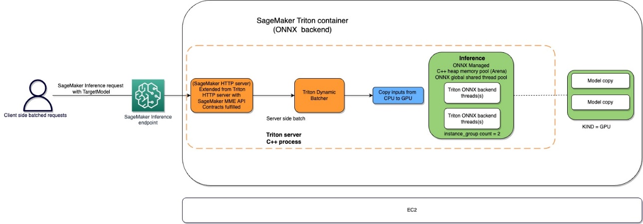
Customers can ship an HTTPS request with the enter payload for real-time inference behind a SageMaker endpoint. The consumer can specify a TargetModel header that incorporates the title of the mannequin that the request in query is destined to invoke. Internally, the SageMaker Triton container implements an HTTP server with the identical contracts as talked about in How Containers Serve Requests. It has help for dynamic batching and helps all of the backends that Triton provides. Based mostly on the configuration, the ONNX runtime is invoked and the request is processed on CPU or GPU as predefined within the mannequin configuration offered by the consumer.

Answer overview

To make use of the ONNX backend, full the next steps:

1. Compile the mannequin to ONNX format.
2. Configure the mannequin.
3. Create the SageMaker endpoint.

Conditions

Guarantee that you’ve entry to an AWS account with enough AWS Identity and Access Management IAM permissions to create a pocket book, entry an Amazon Simple Storage Service (Amazon S3) bucket, and deploy fashions to SageMaker endpoints. See Create execution role for extra data.

Compile the mannequin to ONNX format

The transformers library supplies for handy technique to compile the PyTorch mannequin to ONNX format. The next code achieves the transformations for the NLP mannequin:

onnx_inputs, onnx_outputs = transformers.onnx.export(
    preprocessor=tokenizer,
    mannequin=mannequin,
    config=onnx_config,
    opset=12,
    output=save_path
 )

Exporting fashions (both PyTorch or TensorFlow) is well achieved by way of the conversion device offered as a part of the Hugging Face transformers repository.

The next is what occurs beneath the hood:

1. Allocate the mannequin from transformers (PyTorch or TensorFlow).
2. Ahead dummy inputs by way of the mannequin. This manner, ONNX can report the set of operations run.
3. The transformers inherently care for dynamic axes when exporting the mannequin.
4. Save the graph together with the community parameters.

The same mechanism is adopted for the pc imaginative and prescient use case from the torchvision mannequin zoo:

torch.onnx.export(
        resnet50,
        dummy_input,
        args.save,
        export_params=True,
        opset_version=11,
        do_constant_folding=True,
        input_names=["input"],
        output_names=["output"],
        dynamic_axes={"enter": {0: "batch_size"}, "output": {0: "batch_size"}},
    )

Configure the mannequin

On this part, we configure the pc imaginative and prescient and NLP mannequin. We present tips on how to create a ResNet50 and RoBERTA giant mannequin that has been pre-trained for deployment on a SageMaker MME by using Triton Inference Server mannequin configurations. The ResNet50 pocket book is on the market on GitHub. The RoBERTA pocket book can be accessible on GitHub. For ResNet50, we use the Docker strategy to create an setting that already has all of the dependencies required to construct our ONNX mannequin and generate the mannequin artifacts wanted for this train. This strategy makes it a lot simpler to share dependencies and create the precise setting that’s wanted to perform this process.

Step one is to create the ONNX mannequin package deal per the listing construction laid out in ONNX Models. Our goal is to make use of the minimal mannequin repository for a ONNX mannequin contained in a single file as follows:

<model-repository-path> / 
    Model_name
    ├── 1
    │   └── mannequin.onnx
    └── config.pbtxt

Subsequent, we create the model configuration file that describes the inputs, outputs, and backend configurations for the Triton Server to choose up and invoke the suitable kernels for ONNX. This file is called config.pbtxt and is proven within the following code for the RoBERTA use case. Be aware that the BATCH dimension is omitted from the config.pbtxt. Nevertheless, when sending the information to the mannequin, we embody the batch dimension. The next code additionally exhibits how one can add this function with mannequin configuration information to set dynamic batching with a most popular batch dimension of 5 for the precise inference. With the present settings, the mannequin occasion is invoked immediately when the popular batch dimension of 5 is met or the delay time of 100 microseconds has elapsed for the reason that first request reached the dynamic batcher.

title: "nlp-onnx"
platform: "onnxruntime_onnx"
backend: "onnxruntime" 
max_batch_size: 32

  enter {
    title: "input_ids"
    data_type: TYPE_INT64
    dims: [512]
  }
  enter {
    title: "attention_mask"
    data_type: TYPE_INT64
    dims: [512]
  }

  output {
    title: "last_hidden_state"
    data_type: TYPE_FP32
    dims: [-1, 768]
  }
  output {
    title: "1550"
    data_type: TYPE_FP32
    dims: [768]
  }
instance_group {
  rely: 1
  type: KIND_GPU
}
dynamic_batching {
    max_queue_delay_microseconds: 100
    preferred_batch_size:5
}

The next is the same configuration file for the pc imaginative and prescient use case:

title: "resenet_onnx"
platform: "onnxruntime_onnx"
max_batch_size : 128
enter [
  {
    name: "input"
    data_type: TYPE_FP32
    format: FORMAT_NCHW
    dims: [ 3, 224, 224 ]
  }
]
output [
  {
    name: "output"
    data_type: TYPE_FP32
    dims: [ 1000 ]
  }
]

Create the SageMaker endpoint

We use the Boto3 APIs to create the SageMaker endpoint. For this put up, we present the steps for the RoBERTA pocket book, however these are widespread steps and would be the similar for the ResNet50 mannequin as properly.

Create a SageMaker mannequin

We now create a SageMaker model. We use the Amazon Elastic Container Registry (Amazon ECR) picture and the mannequin artifact from the earlier step to create the SageMaker mannequin.

Create the container

To create the container, we pull the appropriate image from Amazon ECR for Triton Server. SageMaker permits us to customise and inject numerous setting variables. A number of the key options are the power to set the BATCH_SIZE; we will set this per mannequin within the config.pbtxt file, or we will outline a default worth right here. For fashions that may profit from bigger shared reminiscence dimension, we will set these values beneath SHM variables. To allow logging, set the log verbose degree to true. We use the next code to create the mannequin to make use of in our endpoint:

mme_triton_image_uri = (
    f"{account_id_map[region]}.dkr.ecr.{area}.{base}" + "/sagemaker-tritonserver:22.12-py3"
)
container = {
    "Picture": mme_triton_image_uri,
    "ModelDataUrl": mme_path,
    "Mode": "MultiModel",
    "Atmosphere": {
        "SAGEMAKER_TRITON_SHM_DEFAULT_BYTE_SIZE": "16777216000", # "16777216", #"16777216000",
        "SAGEMAKER_TRITON_SHM_GROWTH_BYTE_SIZE": "10485760",
    },
}
from sagemaker.utils import name_from_base
model_name = name_from_base(f"flan-xxl-fastertransformer")
print(model_name)
create_model_response = sm_client.create_model(
    ModelName=model_name,
    ExecutionRoleArn=function,
    PrimaryContainer={
        "Picture": inference_image_uri, 
        "ModelDataUrl": s3_code_artifact
    },
)
model_arn = create_model_response["ModelArn"]
print(f"Created Mannequin: {model_arn}")

Create a SageMaker endpoint

You should use any cases with a number of GPUs for testing. On this put up, we use a g4dn.4xlarge occasion. We don’t set the VolumeSizeInGB parameters as a result of this occasion comes with native occasion storage. The VolumeSizeInGB parameter is relevant to GPU cases supporting the Amazon Elastic Block Store (Amazon EBS) quantity attachment. We will go away the mannequin obtain timeout and container startup well being verify on the default values. For extra particulars, check with CreateEndpointConfig.

endpoint_config_response = sm_client.create_endpoint_config(
EndpointConfigName=endpoint_config_name,
    ProductionVariants=[{
            "VariantName": "AllTraffic",
            "ModelName": model_name,
            "InstanceType": "ml.g4dn.4xlarge",
            "InitialInstanceCount": 1,
            #"VolumeSizeInGB" : 200,
            #"ModelDataDownloadTimeoutInSeconds": 600,
            #"ContainerStartupHealthCheckTimeoutInSeconds": 600,
        },
    ],)'

Lastly, we create a SageMaker endpoint:

create_endpoint_response = sm_client.create_endpoint(
EndpointName=f"{endpoint_name}", EndpointConfigName=endpoint_config_name)

Invoke the mannequin endpoint

This can be a generative mannequin, so we move within the input_ids and attention_mask to the mannequin as a part of the payload. The next code exhibits tips on how to create the tensors:

tokenizer("This can be a pattern", padding="max_length", max_length=max_seq_len)

We now create the suitable payload by guaranteeing the information kind matches what we configured within the config.pbtxt. This additionally give us the tensors with the batch dimension included, which is what Triton expects. We use the JSON format to invoke the mannequin. Triton additionally supplies a local binary invocation technique for the mannequin.

response = runtime_sm_client.invoke_endpoint(
    EndpointName=endpoint_name,
    ContentType="utility/octet-stream",
    Physique=json.dumps(payload),
    TargetModel=f"{tar_file_name}",
    # TargetModel=f"roberta-large-v0.tar.gz",
)

Be aware the TargetModel parameter within the previous code. We ship the title of the mannequin to be invoked as a request header as a result of this can be a multi-model endpoint, subsequently we will invoke a number of fashions at runtime on an already deployed inference endpoint by altering this parameter. This exhibits the facility of multi-model endpoints!

To output the response, we will use the next code:

import numpy as np

resp_bin = response["Body"].learn().decode("utf8")
# -- keys are -- "outputs":[{"name":"1550","datatype":"FP32","shape":[1,768],"information": [0.0013,0,3433...]}]
for information in json.hundreds(resp_bin)["outputs"]:
    shape_1 = listing(information["shape"])
    dat_1 = np.array(information["data"])
    dat_1.resize(shape_1)
    print(f"Information Outputs recieved again :Form:{dat_1.form}")

ONNX for efficiency tuning

The ONNX backend makes use of C++ area reminiscence allocation. Enviornment allocation is a C++-only function that helps you optimize your reminiscence utilization and enhance efficiency. Reminiscence allocation and deallocation constitutes a major fraction of CPU time spent in protocol buffers code. By default, new object creation performs heap allocations for every object, every of its sub-objects, and several other area varieties, reminiscent of strings. These allocations happen in bulk when parsing a message and when constructing new messages in reminiscence, and related deallocations occur when messages and their sub-object timber are freed.

Enviornment-based allocation has been designed to cut back this efficiency price. With area allocation, new objects are allotted out of a big piece of pre-allocated reminiscence known as the area. Objects can all be freed directly by discarding your complete area, ideally with out working destructors of any contained object (although an area can nonetheless preserve a destructor listing when required). This makes object allocation sooner by decreasing it to a easy pointer increment, and makes deallocation virtually free. Enviornment allocation additionally supplies higher cache effectivity: when messages are parsed, they’re extra prone to be allotted in steady reminiscence, which makes traversing messages extra prone to hit sizzling cache traces. The draw back of arena-based allocation is the C++ heap reminiscence can be over-allocated and keep allotted even after the objects are deallocated. This would possibly result in out of reminiscence or excessive CPU reminiscence utilization. To realize the perfect of each worlds, we use the next configurations offered by Triton and ONNX:

• arena_extend_strategy – This parameter refers back to the technique used to develop the reminiscence area with reference to the dimensions of the mannequin. We suggest setting the worth to 1 (= kSameAsRequested), which isn’t a default worth. The reasoning is as follows: the downside of the default area lengthen technique (kNextPowerOfTwo) is that it’d allocate extra reminiscence than wanted, which could possibly be a waste. Because the title suggests, kNextPowerOfTwo (the default) extends the world by an influence of two, whereas kSameAsRequested extends by a dimension that’s the similar because the allocation request every time. kSameAsRequested is suited to superior configurations the place you understand the anticipated reminiscence utilization upfront. In our testing, as a result of we all know the dimensions of fashions is a continuing worth, we will safely select kSameAsRequested.
• gpu_mem_limit – We set the worth to the CUDA reminiscence restrict. To make use of all potential reminiscence, move within the most size_t. It defaults to SIZE_MAX if nothing is specified. We suggest retaining it as default.
• enable_cpu_mem_arena – This permits the reminiscence area on CPU. The world might pre-allocate reminiscence for future utilization. Set this selection to false when you don’t need it. The default is True. If you happen to disable the world, heap reminiscence allocation will take time, so inference latency will enhance. In our testing, we left it as default.
• enable_mem_pattern – This parameter refers back to the inside reminiscence allocation technique primarily based on enter shapes. If the shapes are fixed, we will allow this parameter to generate a reminiscence sample for the long run and avoid wasting allocation time, making it sooner. Use 1 to allow the reminiscence sample and 0 to disable. It’s advisable to set this to 1 when the enter options are anticipated to be the identical. The default worth is 1.
• do_copy_in_default_stream – Within the context of the CUDA execution supplier in ONNX, a compute stream is a sequence of CUDA operations which are run asynchronously on the GPU. The ONNX runtime schedules operations in several streams primarily based on their dependencies, which helps decrease the idle time of the GPU and obtain higher efficiency. We suggest utilizing the default setting of 1 for utilizing the identical stream for copying and compute; nevertheless, you need to use 0 for utilizing separate streams for copying and compute, which could outcome within the system pipelining the 2 actions. In our testing of the ResNet50 mannequin, we used each 0 and 1 however couldn’t discover any considerable distinction between the 2 by way of efficiency and reminiscence consumption of the GPU system.
• Graph optimization – The ONNX backend for Triton helps a number of parameters that assist fine-tune the mannequin dimension in addition to runtime efficiency of the deployed mannequin. When the mannequin is transformed to the ONNX illustration (the primary field within the following diagram on the IR stage), the ONNX runtime supplies graph optimizations at three ranges: primary, prolonged, and structure optimizations. You may activate all ranges of graph optimizations by including the next parameters within the mannequin configuration file:

  optimization {
    graph : {
      degree : 1
  }}

• cudnn_conv_algo_search – As a result of we’re utilizing CUDA-based Nvidia GPUs in our testing, for our laptop imaginative and prescient use case with the ResNet50 mannequin, we will use the CUDA execution provider-based optimization on the fourth layer within the following diagram with the cudnn_conv_algo_search parameter. The default possibility is exhaustive (0), however after we modified this configuration to 1 – HEURISTIC, we noticed the mannequin latency in regular state cut back to 160 milliseconds. The rationale this occurs is as a result of the ONNX runtime invokes the lighter weight cudnnGetConvolutionForwardAlgorithm_v7 ahead move and subsequently reduces latency with satisfactory efficiency.
• Run mode – The following step is choosing the proper execution_mode at layer 5 within the following diagram. This parameter controls whether or not you wish to run operators in your graph sequentially or in parallel. Normally when the mannequin has many branches, setting this selection to ExecutionMode.ORT_PARALLEL (1) offers you higher efficiency. Within the situation the place your mannequin has many branches in its graph, setting the run mode to parallel will assist with higher efficiency. The default mode is sequential, so you’ll be able to allow this to fit your wants.

  parameters { key: "execution_mode" worth: { string_value: "1" } }

For a deeper understanding of the alternatives for efficiency tuning in ONNX, check with the next determine.

Supply: https://static.linaro.org/connect/san19/presentations/san19-211.pdf

Benchmark numbers and efficiency tuning

By turning on the graph optimizations, cudnn_conv_algo_search, and parallel run mode parameters in our testing of the ResNet50 mannequin, we noticed the chilly begin time of the ONNX mannequin graph cut back from 4.4 seconds to 1.61 seconds. An instance of a whole mannequin configuration file is offered within the ONNX configuration part of the next notebook.

The testing benchmark outcomes are as follows:

• PyTorch – 176 milliseconds, chilly begin 6 seconds
• TensorRT – 174 milliseconds, chilly begin 4.5 seconds
• ONNX – 168 milliseconds, chilly begin 4.4 seconds

The next graphs visualize these metrics.

Moreover, in our testing of laptop imaginative and prescient use circumstances, think about sending the request payload in binary format utilizing the HTTP shopper offered by Triton as a result of it considerably improves mannequin invoke latency.

Different parameters that SageMaker exposes for ONNX on Triton are as follows:

• Dynamic batching – Dynamic batching is a function of Triton that enables inference requests to be mixed by the server, so {that a} batch is created dynamically. Making a batch of requests sometimes leads to elevated throughput. The dynamic batcher needs to be used for stateless fashions. The dynamically created batches are distributed to all mannequin cases configured for the mannequin.
• Most batch dimension – The max_batch_size property signifies the utmost batch dimension that the mannequin helps for the types of batching that may be exploited by Triton. If the mannequin’s batch dimension is the primary dimension, and all inputs and outputs to the mannequin have this batch dimension, then Triton can use its dynamic batcher or sequence batcher to robotically use batching with the mannequin. On this case, max_batch_size needs to be set to a price higher than or equal to 1, which signifies the utmost batch dimension that Triton ought to use with the mannequin.
• Default max batch dimension – The default-max-batch-size worth is used for max_batch_size throughout autocomplete when no different worth is discovered. The onnxruntime backend will set the max_batch_size of the mannequin to this default worth if autocomplete has decided the mannequin is able to batching requests and max_batch_size is 0 within the mannequin configuration or max_batch_size is omitted from the mannequin configuration. If max_batch_size is greater than 1 and no scheduler is offered, the dynamic batch scheduler can be used. The default max batch dimension is 4.

Clear up

Be sure that you delete the mannequin, mannequin configuration, and mannequin endpoint after working the pocket book. The steps to do that are offered on the finish of the pattern pocket book within the GitHub repo.

Conclusion

On this put up, we dove deep into the ONNX backend that Triton Inference Server helps on SageMaker. This backend supplies for GPU acceleration of your ONNX fashions. There are numerous choices to think about to get the perfect efficiency for inference, reminiscent of batch sizes, information enter codecs, and different components that may be tuned to satisfy your wants. SageMaker lets you use this functionality utilizing single-model and multi-model endpoints. MMEs enable a greater steadiness of efficiency and price financial savings. To get began with MME help for GPU, see Host multiple models in one container behind one endpoint.

We invite you to strive Triton Inference Server containers in SageMaker, and share your suggestions and questions within the feedback.

Concerning the authors

Abhi Shivaditya is a Senior Options Architect at AWS, working with strategic world enterprise organizations to facilitate the adoption of AWS providers in areas reminiscent of Synthetic Intelligence, distributed computing, networking, and storage. His experience lies in Deep Studying within the domains of Pure Language Processing (NLP) and Pc Imaginative and prescient. Abhi assists clients in deploying high-performance machine studying fashions effectively throughout the AWS ecosystem.

James Park is a Options Architect at Amazon Internet Providers. He works with Amazon.com to design, construct, and deploy expertise options on AWS, and has a specific curiosity in AI and machine studying. In h is spare time he enjoys in search of out new cultures, new experiences,  and staying updated with the newest expertise developments.You’ll find him on LinkedIn.

Rupinder Grewal is a Sr Ai/ML Specialist Options Architect with AWS. He at present focuses on serving of fashions and MLOps on SageMaker. Previous to this function he has labored as Machine Studying Engineer constructing and internet hosting fashions. Exterior of labor he enjoys taking part in tennis and biking on mountain trails.

Dhawal Patel is a Principal Machine Studying Architect at AWS. He has labored with organizations starting from giant enterprises to mid-sized startups on issues associated to distributed computing, and Synthetic Intelligence. He focuses on Deep studying together with NLP and Pc Imaginative and prescient domains. He helps clients obtain excessive efficiency mannequin inference on SageMaker.