
Within the first part of this mini-series on autoregressive flow models, we checked out bijectors in TensorFlow Chance (TFP), and noticed the way to use them for sampling and density estimation. We singled out the affine bijector to show the mechanics of movement development: We begin from a distribution that’s straightforward to pattern from, and that permits for easy calculation of its density. Then, we connect some variety of invertible transformations, optimizing for data-likelihood below the ultimate remodeled distribution. The effectivity of that (log)chance calculation is the place normalizing flows excel: Loglikelihood below the (unknown) goal distribution is obtained as a sum of the density below the bottom distribution of the inverse-transformed information plus absolutely the log determinant of the inverse Jacobian.
Now, an affine movement will seldom be highly effective sufficient to mannequin nonlinear, advanced transformations. In constrast, autoregressive fashions have proven substantive success in density estimation in addition to pattern technology. Mixed with extra concerned architectures, characteristic engineering, and intensive compute, the idea of autoregressivity has powered – and is powering – state-of-the-art architectures in areas reminiscent of picture, speech and video modeling.
This publish shall be involved with the constructing blocks of autoregressive flows in TFP. Whereas we received’t precisely be constructing state-of-the-art fashions, we’ll attempt to perceive and play with some main elements, hopefully enabling the reader to do her personal experiments on her personal information.
This publish has three elements: First, we’ll have a look at autoregressivity and its implementation in TFP. Then, we attempt to (roughly) reproduce one of many experiments within the “MAF paper” (Masked Autoregressive Flows for Distribution Estimation (Papamakarios, Pavlakou, and Murray 2017)) – primarily a proof of idea. Lastly, for the third time on this weblog, we come again to the duty of analysing audio information, with blended outcomes.
Autoregressivity and masking
In distribution estimation, autoregressivity enters the scene through the chain rule of chance that decomposes a joint density right into a product of conditional densities:
[
p(mathbf{x}) = prod_{i}p(mathbf{x}_i|mathbf{x}_{1:i−1})
]
In apply, because of this autoregressive fashions need to impose an order on the variables – an order which could or may not “make sense.” Approaches right here embrace selecting orderings at random and/or utilizing completely different orderings for every layer.
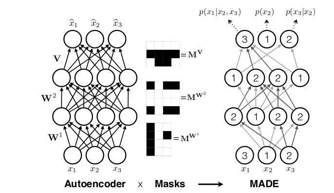
Whereas in recurrent neural networks, autoregressivity is conserved because of the recurrence relation inherent in state updating, it isn’t clear a priori how autoregressivity is to be achieved in a densely related structure. A computationally environment friendly resolution was proposed in MADE: Masked Autoencoder for Distribution Estimation(Germain et al. 2015): Ranging from a densely related layer, masks out all connections that shouldn’t be allowed, i.e., all connections from enter characteristic (i) to stated layer’s activations (1 … i-1). Or expressed in another way, activation (i) could also be related to enter options (1 … i-1) solely. Then when including extra layers, care should be taken to make sure that all required connections are masked in order that on the finish, output (i) will solely ever have seen inputs (1 … i-1).
Thus masked autoregressive flows are a fusion of two main approaches – autoregressive fashions (which needn’t be flows) and flows (which needn’t be autoregressive). In TFP these are offered by MaskedAutoregressiveFlow, for use as a bijector in a TransformedDistribution.
Whereas the documentation exhibits the way to use this bijector, the step from theoretical understanding to coding a “black field” could appear vast. In the event you’re something just like the creator, right here you may really feel the urge to “look below the hood” and confirm that issues actually are the way in which you’re assuming. So let’s give in to curiosity and permit ourselves a bit escapade into the supply code.
Peeking forward, that is how we’ll assemble a masked autoregressive movement in TFP (once more utilizing the nonetheless new-ish R bindings offered by tfprobability):
library(tfprobability)

maf <- tfb_masked_autoregressive_flow(
    shift_and_log_scale_fn = tfb_masked_autoregressive_default_template(
      hidden_layers = list(num_hidden, num_hidden),
      activation = tf$nn$tanh)
)
Pulling aside the related entities right here, tfb_masked_autoregressive_flow is a bijector, with the standard strategies tfb_forward(), tfb_inverse(), tfb_forward_log_det_jacobian() and tfb_inverse_log_det_jacobian().
The default shift_and_log_scale_fn, tfb_masked_autoregressive_default_template, constructs a bit neural community of its personal, with a configurable variety of hidden models per layer, a configurable activation operate and optionally, different configurable parameters to be handed to the underlying dense layers. It’s these dense layers that need to respect the autoregressive property. Can we check out how that is executed? Sure we will, offered we’re not afraid of a bit Python.
masked_autoregressive_default_template (now leaving out the tfb_ as we’ve entered Python-land) makes use of masked_dense to do what you’d suppose a thus-named operate is likely to be doing: assemble a dense layer that has a part of the load matrix masked out. How? We’ll see after a number of Python setup statements.
import numpy as np
import tensorflow as tf
import tensorflow_probability as tfp
tfd = tfp.distributions
tfb = tfp.bijectors
tf.enable_eager_execution()
The following code snippets are taken from masked_dense (in its current form on master), and when potential, simplified for higher readability, accommodating simply the specifics of the chosen instance – a toy matrix of form 2×3:
# construct some toy input data (this line obviously not from the original code)
inputs = tf.constant(np.arange(1.,7), shape = (2, 3))

# (partly) determine shape of mask from shape of input
input_depth = tf.compat.dimension_value(inputs.shape.with_rank_at_least(1)[-1])
num_blocks = input_depth
num_blocks # 3
Our toy layer should have 4 units:
The mask is initialized to all zeros. Considering it will be used to elementwise multiply the weight matrix, we’re a bit surprised at its shape (shouldn’t it be the other way round?). No worries; all will turn out correct in the end.
mask = np.zeros([units, input_depth], dtype=tf.float32.as_numpy_dtype())
mask
array([[0., 0., 0.],
[0., 0., 0.],
[0., 0., 0.],
[0., 0., 0.]], dtype=float32)Now to “whitelist” the allowed connections, we have to fill in ones whenever information flow is allowed by the autoregressive property:
def _gen_slices(num_blocks, n_in, n_out):
  slices = []
  col = 0
  d_in = n_in // num_blocks
  d_out = n_out // num_blocks
  row = d_out
  for _ in range(num_blocks):
    row_slice = slice(row, None)
    col_slice = slice(col, col + d_in)
    slices.append([row_slice, col_slice])
    col += d_in
    row += d_out
  return slices

slices = _gen_slices(num_blocks, input_depth, units)
for [row_slice, col_slice] in slices:
  mask[row_slice, col_slice] = 1

mask
array([[0., 0., 0.],
[1., 0., 0.],
[1., 1., 0.],
[1., 1., 1.]], dtype=float32)Again, does this look mirror-inverted? A transpose fixes shape and logic both:
array([[0., 1., 1., 1.],
       [0., 0., 1., 1.],
       [0., 0., 0., 1.]], dtype=float32)
Now that we have the mask, we can create the layer (interestingly, as of this writing not (yet?) a tf.keras layer):
layer = tf.compat.v1.layers.Dense(
        units,
        kernel_initializer=masked_initializer, # 1
        kernel_constraint=lambda x: mask * x   # 2
        )
Here we see masking going on in two ways. For one, the weight initializer is masked:
kernel_initializer = tf.compat.v1.glorot_normal_initializer()

def masked_initializer(shape, dtype=None, partition_info=None):
 return mask * kernel_initializer(shape, dtype, partition_info)
And secondly, a kernel constraint makes sure that after optimization, the relative units are zeroed out again:
kernel_constraint=lambda x: mask * x Just for fun, let’s apply the layer to our toy input:
<tf.Tensor: id=30, shape=(2, 4), dtype=float64, numpy=
array([[ 0.        , -0.7489589 , -0.43329933,  1.42710014],
       [ 0.        , -2.9958356 , -1.71647246,  1.09258015]])>
Zeroes where expected. And double-checking on the weight matrix…
<tf.Variable 'dense/kernel:0' shape=(3, 4) dtype=float64, numpy=
array([[ 0.        , -0.7489589 , -0.42214942, -0.6473454 ],
       [-0.        ,  0.        , -0.00557496, -0.46692933],
       [-0.        , -0.        , -0.        ,  1.00276807]])>
Good. Now hopefully after this little deep dive, things have become a bit more concrete. Of course in a bigger model, the autoregressive property has to be conserved between layers as well.
On to the second topic, application of MAF to a real-world dataset.
Masked Autoregressive Flow
The MAF paper(Papamakarios, Pavlakou, and Murray 2017) utilized masked autoregressive flows (in addition to single-layer-MADE(Germain et al. 2015) and Actual NVP (Dinh, Sohl-Dickstein, and Bengio 2016)) to a lot of datasets, together with MNIST, CIFAR-10 and several other datasets from the UCI Machine Learning Repository.
We decide one of many UCI datasets: Gas sensors for home activity monitoring. On this dataset, the MAF authors obtained the very best outcomes utilizing a MAF with 10 flows, so that is what we are going to attempt.
Gathering data from the paper, we all know that
- information was included from the file ethylene_CO.txt solely;
- discrete columns had been eradicated, in addition to all columns with correlations > .98; and
- the remaining 8 columns had been standardised (z-transformed).
Concerning the neural community structure, we collect that
- every of the ten MAF layers was adopted by a batchnorm;
- as to characteristic order, the primary MAF layer used the variable order that got here with the dataset; then each consecutive layer reversed it;
- particularly for this dataset and versus all different UCI datasets, tanh was used for activation as a substitute of relu;
- the Adam optimizer was used, with a studying fee of 1e-4;
- there have been two hidden layers for every MAF, with 100 models every;
- coaching went on till no enchancment occurred for 30 consecutive epochs on the validation set; and
- the bottom distribution was a multivariate Gaussian.
That is all helpful data for our try to estimate this dataset, however the important bit is that this. In case you knew the dataset already, you may need been questioning how the authors would take care of the dimensionality of the info: It’s a time sequence, and the MADE structure explored above introduces autoregressivity between options, not time steps. So how is the extra temporal autoregressivity to be dealt with? The reply is: The time dimension is actually eliminated. Within the authors’ phrases,
[…] it’s a time sequence however was handled as if every instance had been an i.i.d. pattern from the marginal distribution.
This undoubtedly is helpful data for our current modeling try, however it additionally tells us one thing else: We’d need to look past MADE layers for precise time sequence modeling.
Now although let’s have a look at this instance of utilizing MAF for multivariate modeling, with no time or spatial dimension to be taken into consideration.
Following the hints the authors gave us, that is what we do.
Observations: 4,208,261
Variables: 19
$ X1  <dbl> 0.00, 0.01, 0.01, 0.03, 0.04, 0.05, 0.06, 0.07, 0.07, 0.09,...
$ X2  <dbl> 0, 0, 0, 0, 0, 0, 0, 0, 0, 0, 0, 0, 0, 0, 0, 0, 0, 0, 0, 0,...
$ X3  <dbl> 0, 0, 0, 0, 0, 0, 0, 0, 0, 0, 0, 0, 0, 0, 0, 0, 0, 0, 0, 0,...
$ X4  <dbl> -50.85, -49.40, -40.04, -47.14, -33.58, -48.59, -48.27, -47.14,...
$ X5  <dbl> -1.95, -5.53, -16.09, -10.57, -20.79, -11.54, -9.11, -4.56,...
$ X6  <dbl> -41.82, -42.78, -27.59, -32.28, -33.25, -36.16, -31.31, -16.57,...
$ X7  <dbl> 1.30, 0.49, 0.00, 4.40, 6.03, 6.03, 5.37, 4.40, 23.98, 2.77,...
$ X8  <dbl> -4.07, 3.58, -7.16, -11.22, 3.42, 0.33, -7.97, -2.28, -2.12,...
$ X9  <dbl> -28.73, -34.55, -42.14, -37.94, -34.22, -29.05, -30.34, -24.35,...
$ X10 <dbl> -13.49, -9.59, -12.52, -7.16, -14.46, -16.74, -8.62, -13.17,...
$ X11 <dbl> -3.25, 5.37, -5.86, -1.14, 8.31, -1.14, 7.00, -6.34, -0.81,...
$ X12 <dbl> 55139.95, 54395.77, 53960.02, 53047.71, 52700.28, 51910.52,...
$ X13 <dbl> 50669.50, 50046.91, 49299.30, 48907.00, 48330.96, 47609.00,...
$ X14 <dbl> 9626.26, 9433.20, 9324.40, 9170.64, 9073.64, 8982.88, 8860.51,...
$ X15 <dbl> 9762.62, 9591.21, 9449.81, 9305.58, 9163.47, 9021.08, 8966.48,...
$ X16 <dbl> 24544.02, 24137.13, 23628.90, 23101.66, 22689.54, 22159.12,...
$ X17 <dbl> 21420.68, 20930.33, 20504.94, 20101.42, 19694.07, 19332.57,...
$ X18 <dbl> 7650.61, 7498.79, 7369.67, 7285.13, 7156.74, 7067.61, 6976.13,...
$ X19 <dbl> 6928.42, 6800.66, 6697.47, 6578.52, 6468.32, 6385.31, 6300.97,...
# A tibble: 4,208,261 x 8
X4 X5 X8 X9 X13 X16 X17 X18
<dbl> <dbl> <dbl> <dbl> <dbl> <dbl> <dbl> <dbl>
1 -50.8 -1.95 -4.07 -28.7 50670. 24544. 21421. 7651.
2 -49.4 -5.53 3.58 -34.6 50047. 24137. 20930. 7499.
3 -40.0 -16.1 -7.16 -42.1 49299. 23629. 20505. 7370.
4 -47.1 -10.6 -11.2 -37.9 48907 23102. 20101. 7285.
5 -33.6 -20.8 3.42 -34.2 48331. 22690. 19694. 7157.
6 -48.6 -11.5 0.33 -29.0 47609 22159. 19333. 7068.
7 -48.3 -9.11 -7.97 -30.3 47047. 21932. 19028. 6976.
8 -47.1 -4.56 -2.28 -24.4 46758. 21504. 18780. 6900.
9 -42.3 -2.77 -2.12 -27.6 46197. 21125. 18439. 6827.
10 -44.6 3.58 -0.65 -35.5 45652. 20836. 18209. 6790.
# … with 4,208,251 extra rowsNow arrange the info technology course of:
# train-test break up
n_rows <- nrow(df2) # 4208261
train_ids <- sample(1:n_rows, 0.5 * n_rows)
x_train <- df2[train_ids, ]
x_test <- df2[-train_ids, ]

# create datasets
batch_size <- 100
train_dataset <- tf$solid(x_train, tf$float32) %>%
  tensor_slices_dataset %>%
  dataset_batch(batch_size)

test_dataset <- tf$solid(x_test, tf$float32) %>%
  tensor_slices_dataset %>%
  dataset_batch(nrow(x_test))
To assemble the movement, the very first thing wanted is the bottom distribution.
Now for the movement, by default constructed with batchnorm and permutation of characteristic order.
num_hidden <- 100
dim <- ncol(df2)

use_batchnorm <- TRUE
use_permute <- TRUE
num_mafs <-10
num_layers <- 3 * num_mafs

bijectors <- vector(mode = "record", size = num_layers)

for (i in seq(1, num_layers, by = 3)) {
  maf <- tfb_masked_autoregressive_flow(
    shift_and_log_scale_fn = tfb_masked_autoregressive_default_template(
      hidden_layers = list(num_hidden, num_hidden),
      activation = tf$nn$tanh))
  bijectors[[i]] <- maf
  if (use_batchnorm)
    bijectors[[i + 1]] <- tfb_batch_normalization()
  if (use_permute)
    bijectors[[i + 2]] <- tfb_permute((ncol(df2) - 1):0)
}

if (use_permute) bijectors <- bijectors[-num_layers]

movement <- bijectors %>%
  discard(is.null) %>%
  # tfb_chain expects arguments in reverse order of software
  rev() %>%
  tfb_chain()

target_dist <- tfd_transformed_distribution(
  distribution = base_dist,
  bijector = movement
)
And configuring the optimizer:
optimizer <- tf$practice$AdamOptimizer(1e-4)Beneath that isotropic Gaussian we selected as a base distribution, how doubtless are the info?
base_loglik <- base_dist %>%
  tfd_log_prob(x_train) %>%
  tf$reduce_mean()
base_loglik %>% as.numeric()        # -11.33871

base_loglik_test <- base_dist %>%
  tfd_log_prob(x_test) %>%
  tf$reduce_mean()
base_loglik_test %>% as.numeric()   # -11.36431
And, simply as a fast sanity verify: What’s the loglikelihood of the info below the remodeled distribution earlier than any coaching?
target_loglik_pre <-
  target_dist %>% tfd_log_prob(x_train) %>% tf$reduce_mean()
target_loglik_pre %>% as.numeric()        # -11.22097

target_loglik_pre_test <-
  target_dist %>% tfd_log_prob(x_test) %>% tf$reduce_mean()
target_loglik_pre_test %>% as.numeric()   # -11.36431
The values match – good. Right here now’s the coaching loop. Being impatient, we already preserve checking the loglikelihood on the (full) take a look at set to see if we’re making any progress.
n_epochs <- 10

for (i in 1:n_epochs) {

  agg_loglik <- 0
  num_batches <- 0
  iter <- make_iterator_one_shot(train_dataset)

  until_out_of_range({
    batch <- iterator_get_next(iter)
    loss <-
      operate()
        - tf$reduce_mean(target_dist %>% tfd_log_prob(batch))
    optimizer$reduce(loss)

    loglik <- tf$reduce_mean(target_dist %>% tfd_log_prob(batch))
    agg_loglik <- agg_loglik + loglik
    num_batches <- num_batches + 1

    test_iter <- make_iterator_one_shot(test_dataset)
    test_batch <- iterator_get_next(test_iter)
    loglik_test_current <- target_dist %>% tfd_log_prob(test_batch) %>% tf$reduce_mean()

    if (num_batches %% 100 == 1)
      cat(
        "Epoch ",
        i,
        ": ",
        "Batch ",
        num_batches,
        ": ",
        (agg_loglik %>% as.numeric()) / num_batches,
        " --- take a look at: ",
        loglik_test_current %>% as.numeric(),
        "n"
      )
  })
}
With each coaching and take a look at units amounting to over 2 million information every, we didn’t have the endurance to run this mannequin till no enchancment occurred for 30 consecutive epochs on the validation set (just like the authors did). Nevertheless, the image we get from one full epoch’s run is fairly clear: The setup appears to work fairly okay.
Epoch  1 :  Batch      1:  -8.212026  --- take a look at:  -10.09264
Epoch  1 :  Batch   1001:   2.222953  --- take a look at:   1.894102
Epoch  1 :  Batch   2001:   2.810996  --- take a look at:   2.147804
Epoch  1 :  Batch   3001:   3.136733  --- take a look at:   3.673271
Epoch  1 :  Batch   4001:   3.335549  --- take a look at:   4.298822
Epoch  1 :  Batch   5001:   3.474280  --- take a look at:   4.502975
Epoch  1 :  Batch   6001:   3.606634  --- take a look at:   4.612468
Epoch  1 :  Batch   7001:   3.695355  --- take a look at:   4.146113
Epoch  1 :  Batch   8001:   3.767195  --- take a look at:   3.770533
Epoch  1 :  Batch   9001:   3.837641  --- take a look at:   4.819314
Epoch  1 :  Batch  10001:   3.908756  --- take a look at:   4.909763
Epoch  1 :  Batch  11001:   3.972645  --- take a look at:   3.234356
Epoch  1 :  Batch  12001:   4.020613  --- take a look at:   5.064850
Epoch  1 :  Batch  13001:   4.067531  --- take a look at:   4.916662
Epoch  1 :  Batch  14001:   4.108388  --- take a look at:   4.857317
Epoch  1 :  Batch  15001:   4.147848  --- take a look at:   5.146242
Epoch  1 :  Batch  16001:   4.177426  --- take a look at:   4.929565
Epoch  1 :  Batch  17001:   4.209732  --- take a look at:   4.840716
Epoch  1 :  Batch  18001:   4.239204  --- take a look at:   5.222693
Epoch  1 :  Batch  19001:   4.264639  --- take a look at:   5.279918
Epoch  1 :  Batch  20001:   4.291542  --- take a look at:   5.29119
Epoch  1 :  Batch  21001:   4.314462  --- take a look at:   4.872157
Epoch  2 :  Batch      1:   5.212013  --- take a look at:   4.969406
With these coaching outcomes, we regard the proof of idea as mainly profitable. Nevertheless, from our experiments we additionally need to say that the selection of hyperparameters appears to matter a lot. For instance, use of the relu activation operate as a substitute of tanh resulted within the community mainly studying nothing. (As per the authors, relu labored effective on different datasets that had been z-transformed in simply the identical means.)
Batch normalization right here was compulsory – and this may go for flows typically. The permutation bijectors, alternatively, didn’t make a lot of a distinction on this dataset. Total the impression is that for flows, we’d both want a “bag of methods” (like is often stated about GANs), or extra concerned architectures (see “Outlook” under).
Lastly, we wind up with an experiment, coming again to our favourite audio information, already featured in two posts: Simple Audio Classification with Keras and Audio classification with Keras: Looking closer at the non-deep learning parts.
Analysing audio information with MAF
The dataset in question consists of recordings of 30 phrases, pronounced by a lot of completely different audio system. In these earlier posts, a convnet was skilled to map spectrograms to these 30 courses. Now as a substitute we wish to attempt one thing completely different: Prepare an MAF on one of many courses – the phrase “zero,” say – and see if we will use the skilled community to mark “non-zero” phrases as much less doubtless: carry out anomaly detection, in a means. Spoiler alert: The outcomes weren’t too encouraging, and in case you are excited by a process like this, you may wish to contemplate a distinct structure (once more, see “Outlook” under).
Nonetheless, we rapidly relate what was executed, as this process is a pleasant instance of dealing with information the place options differ over a couple of axis.
Preprocessing begins as within the aforementioned earlier posts. Right here although, we explicitly use keen execution, and will typically hard-code identified values to maintain the code snippets brief.
library(tensorflow)
library(tfprobability)

tfe_enable_eager_execution(device_policy = "silent")

library(tfdatasets)
library(dplyr)
library(readr)
library(purrr)
library(caret)
library(stringr)

# make decode_wav() run with the current release 1.13.1 as well as with the current master branch
decode_wav <- function() if (reticulate::py_has_attr(tf, "audio")) tf$audio$decode_wav
  else tf$contrib$framework$python$ops$audio_ops$decode_wav
# same for stft()
stft <- function() if (reticulate::py_has_attr(tf, "signal")) tf$signal$stft else tf$spectral$stft

files <- fs::dir_ls(path = "audio/data_1/speech_commands_v0.01/", # replace by yours
                    recursive = TRUE,
                    glob = "*.wav")

files <- files[!str_detect(files, "background_noise")]

df <- tibble(
  fname = files,
  class = fname %>%
    str_extract("v0.01/.*/") %>%
    str_replace_all("v0.01/", "") %>%
    str_replace_all("/", "")
)
We train the MAF on pronunciations of the word “zero.”
Following the approach detailed in Audio classification with Keras: Looking closer at the non-deep learning parts, we’d like to coach the community on spectrograms as a substitute of the uncooked time area information.
Utilizing the identical settings for frame_length and frame_step of the Brief Time period Fourier Remodel as in that publish, we’d arrive at information formed variety of frames x variety of FFT coefficients. To make this work with the masked_dense() employed in tfb_masked_autoregressive_flow(), the info would then need to be flattened, yielding a powerful 25186 options within the joint distribution.
With the structure outlined as above within the GAS instance, this result in the community not making a lot progress. Neither did leaving the info in time area kind, with 16000 options within the joint distribution. Thus, we determined to work with the FFT coefficients computed over the whole window as a substitute, leading to 257 joint options.
batch_size <- 100

sampling_rate <- 16000L
data_generator <- operate(df,
                           batch_size) {

  ds <- tensor_slices_dataset(df)

  ds <- ds %>%
    dataset_map(operate(obs) {
      wav <-
        decode_wav()(tf$read_file(tf$reshape(obs$fname, list())))
      samples <- wav$audio[ ,1]

      # some wave recordsdata have fewer than 16000 samples
      padding <- list(list(0L, sampling_rate - tf$form(samples)[1]))
      padded <- tf$pad(samples, padding)

      stft_out <- stft()(padded, 16000L, 1L, 512L)
      magnitude_spectrograms <- tf$abs(stft_out) %>% tf$squeeze()
    })

  ds %>% dataset_batch(batch_size)

}

ds_train <- data_generator(df_train, batch_size)
batch <- ds_train %>%
  make_iterator_one_shot() %>%
  iterator_get_next()

dim(batch) # 100 x 257
Coaching then proceeded as on the GAS dataset.
# outline MAF
base_dist <-
  tfd_multivariate_normal_diag(loc = rep(0, dim(batch)[2]))

num_hidden <- 512
use_batchnorm <- TRUE
use_permute <- TRUE
num_mafs <- 10
num_layers <- 3 * num_mafs

# retailer bijectors in a listing
bijectors <- vector(mode = "record", size = num_layers)

# fill record, optionally including batchnorm and permute bijectors
for (i in seq(1, num_layers, by = 3)) {
  maf <- tfb_masked_autoregressive_flow(
    shift_and_log_scale_fn = tfb_masked_autoregressive_default_template(
      hidden_layers = list(num_hidden, num_hidden),
      activation = tf$nn$tanh,
      ))
  bijectors[[i]] <- maf
  if (use_batchnorm)
    bijectors[[i + 1]] <- tfb_batch_normalization()
  if (use_permute)
    bijectors[[i + 2]] <- tfb_permute((dim(batch)[2] - 1):0)
}

if (use_permute) bijectors <- bijectors[-num_layers]
movement <- bijectors %>%
  # probably clear out empty parts (if no batchnorm or no permute)
  discard(is.null) %>%
  rev() %>%
  tfb_chain()

target_dist <- tfd_transformed_distribution(distribution = base_dist,
                                            bijector = movement)

optimizer <- tf$practice$AdamOptimizer(1e-3)

# practice MAF
n_epochs <- 100
for (i in 1:n_epochs) {
  agg_loglik <- 0
  num_batches <- 0
  iter <- make_iterator_one_shot(ds_train)
  until_out_of_range({
    batch <- iterator_get_next(iter)
    loss <-
      operate()
        - tf$reduce_mean(target_dist %>% tfd_log_prob(batch))
    optimizer$reduce(loss)

    loglik <- tf$reduce_mean(target_dist %>% tfd_log_prob(batch))
    agg_loglik <- agg_loglik + loglik
    num_batches <- num_batches + 1

    loglik_test_current <-
      target_dist %>% tfd_log_prob(ds_test) %>% tf$reduce_mean()

    if (num_batches %% 20 == 1)
      cat(
        "Epoch ",
        i,
        ": ",
        "Batch ",
        num_batches,
        ": ",
        ((agg_loglik %>% as.numeric()) / num_batches) %>% round(1),
        " --- take a look at: ",
        loglik_test_current %>% as.numeric() %>% round(1),
        "n"
      )
  })
}
Throughout coaching, we additionally monitored loglikelihoods on three completely different courses, cat, hen and wow. Listed below are the loglikelihoods from the primary 10 epochs. “Batch” refers back to the present coaching batch (first batch within the epoch), all different values refer to finish datasets (the whole take a look at set and the three units chosen for comparability).
epoch   |   batch  |   take a look at   |   "cat"  |   "hen"  |   "wow"  |
--------|----------|----------|----------|-----------|----------|
1       |   1443.5 |   1455.2 |   1398.8 |    1434.2 |   1546.0 |
2       |   1935.0 |   2027.0 |   1941.2 |    1952.3 |   2008.1 |
3       |   2004.9 |   2073.1 |   2003.5 |    2000.2 |   2072.1 |
4       |   2063.5 |   2131.7 |   2056.0 |    2061.0 |   2116.4 |
5       |   2120.5 |   2172.6 |   2096.2 |    2085.6 |   2150.1 |
6       |   2151.3 |   2206.4 |   2127.5 |    2110.2 |   2180.6 |
7       |   2174.4 |   2224.8 |   2142.9 |    2163.2 |   2195.8 |
8       |   2203.2 |   2250.8 |   2172.0 |    2061.0 |   2221.8 |
9       |   2224.6 |   2270.2 |   2186.6 |    2193.7 |   2241.8 |
10      |   2236.4 |   2274.3 |   2191.4 |    2199.7 |   2243.8 |
Whereas this doesn’t look too dangerous, a whole comparability towards all twenty-nine non-target courses had “zero” outperformed by seven different courses, with the remaining twenty-two decrease in loglikelihood. We don’t have a mannequin for anomaly detection, as but.
Outlook
As already alluded to a number of instances, for information with temporal and/or spatial orderings extra advanced architectures could show helpful. The very profitable PixelCNN household is predicated on masked convolutions, with more moderen developments bringing additional refinements (e.g. Gated PixelCNN (Oord et al. 2016), PixelCNN++ (Salimans et al. 2017). Consideration, too, could also be masked and thus rendered autoregressive, as employed within the hybrid PixelSNAIL (Chen et al. 2017) and the – not surprisingly given its identify – transformer-based ImageTransformer (Parmar et al. 2018).
To conclude, – whereas this publish was within the intersection of flows and autoregressivity – and final not least the use therein of TFP bijectors – an upcoming one may dive deeper into autoregressive fashions particularly… and who is aware of, maybe come again to the audio information for a fourth time.

