Creating an Infographic With Matplotlib | by Andy McDonald | Jul, 2023

So, primarily based on that, I assumed to myself, why not strive constructing an infographic with matplotlib.

And I did.

The next infographic was the results of that, and it’s what we might be recreating on this article.

Keep in mind that the infographic we might be constructing on this article could also be appropriate for internet use or included inside a presentation. Nonetheless, if we have been trying to embrace these inside stories or show them in additional formal settings, we might wish to think about different color palettes and a extra skilled really feel.

Earlier than we contact any knowledge visualisation, we have to perceive the aim behind creating our infographic. With out this, will probably be difficult to slim down the plots we wish to use and the story we wish to inform.

For this instance, we’re going to use a set of effectively log derived lithology measurements which were obtained from the Norwegian Continental Shelf. From this dataset, we’re going to particularly take a look at the query:

What’s the lithological variation of the Zechstein Group inside this dataset?

This offers us with our place to begin.

We all know that we’re on the lookout for lithology knowledge and knowledge throughout the Zechstein Group.

To start, we first have to import quite a few key libraries.

These are pandas, for loading and storing our knowledge, numpy for performing mathematical calculations to permit us to plot labels and knowledge in a polar projections, matplotlib for creating our plot, and adjustText to make sure labels don’t overlap on our scatter plot.

import pandas as pd
import matplotlib.pyplot as plt
import numpy as np
from adjustText import adjust_text

After the libraries have been imported, we subsequent have to load our datasets. Particulars of the supply for this dataset is included on the backside of this text.

The primary dataset we’ll load is the lithology composition of the Zechstein Group created in my previous article.

We are able to load this knowledge in utilizing pandas read_csv() operate.

df = pd.read_csv('Knowledge/LithologySummary.csv', index_col='WELL')

After we view our dataframe we now have the next details about the lithologies current throughout the Zechstein Group as interpreted inside every effectively.

To assist our readers perceive the info higher, it will be good to have details about the place the drilled wells intersected with the Zechstein Group.

We are able to load this knowledge in the identical approach by utilizing pd.read_csv(). Nonetheless, this time, we don’t have to set an index.

zechstein_well_intersections = pd.read_csv('Knowledge/Zechstein_WellIntersection.csv')

After we view this dataframe we’re introduced with the next desk containing the effectively identify, the X & Y grid areas of the place the effectively penetrated the Zechstein Group.

Earlier than we start creating any figures, we have to create a number of variables containing key details about our knowledge. This may make issues simpler on the subject of making the plots.

First, we’ll get a listing of all the attainable lithologies. That is carried out by changing the column names inside our abstract dataframe to a listing.

lith_names = record(df.columns)

After we view this record, we get again the next lithologies.

Subsequent, we have to determine how we wish the person plots throughout the infographic to be arrange.

For this dataset, we now have 8 wells, which might be used to generate 8 radial bar charts.

We additionally wish to present effectively areas on the identical determine as effectively. So this provides us 9 subplots.

A method we will subdivide our determine is to have 3 columns and three rows. This enables us to create our first variable, num_cols representing the variety of columns.

We are able to then generalise the variety of rows ( num_rows ) variable in order that we will reuse it with different datasets. On this instance, it’s going to take the variety of wells we now have (the variety of rows within the dataframe) and divide it by the variety of columns we wish. Utilizing np.ceil will permit us to spherical this quantity up in order that we now have all the plots on the determine.

# Set the variety of columns to your subplot grid
num_cols = 3
# Get the variety of wells (rows within the DataFrame)
num_wells = len(df)
# Calculate the variety of rows wanted for the subplot grid
num_rows = np.ceil(num_wells / num_cols).astype(int)

The subsequent set of variables we have to declare are as follows:

• indexes : creates a listing of numbers starting from 0 to the overall variety of gadgets in our record. In our case, it will generate a listing from 0 to 7, which covers the 8 lithologies in our dataset.
• width : creates a listing primarily based on calculating the width of every bar within the chart by dividing the circumference of a circle by the variety of rock varieties we now have in rock_names
• angles : creates a listing containing the angles for every of the rock varieties
• colors : a listing of hexadecimal colors we wish to use to characterize every effectively
• label_loc : creates a listing of evenly spaced values between 0 and a couple of * pi for displaying the rock-type labels

indexes = record(vary(0, len(lith_names)))
width = 2*np.pi / len(lith_names)
angles = [element * width for element in indexes]
colors = ["#ae1241", "#5ba8f7", "#c6a000", "#0050ae", 
"#9b54f3", "#ff7d67", "#dbc227", "#008c5c"]
label_loc = np.linspace(begin=0, cease=2 * np.pi, num=len(lith_names))

Including Radial Bar Charts as Subplots

To start creating our infographic, we first have to create a determine object. That is carried out by calling upon plt.determine().

To setup our determine, we have to cross in a number of parameters:

• figsize : controls the scale of the infographic. As we might have various numbers of rows, we will set the rows parameter to be a a number of of the variety of rows. This may stop the plots and figures from changing into distorted.
• linewidth : controls the border thickness for the determine
• edgecolor : units the border color
• facecolor : units the determine background color

# Create a determine
fig = plt.determine(figsize=(20, num_rows * 7), linewidth=10,
edgecolor='#393d5c', 
facecolor='#25253c')

Subsequent, we have to outline our grid structure. There are a number of methods we will do that, however for this instance, we’re going to use GridSpec. This may permit us to specify the placement of the subplots, and in addition the spacing between them.

# Create a grid structure
grid = plt.GridSpec(num_rows, num_cols, wspace=0.5, hspace=0.5)

We at the moment are prepared to start including our radial bar plots.

To do that, we have to loop over every row throughout the lithology composition abstract dataframe and add an axis to the grid utilizing add_subplot() As we’re plotting radial bar charts, we wish to set the projection parameter to polar.

Subsequent, we will start including our knowledge to the plot by calling upon ax.bar. Inside this name, we cross in:

• angles : offers the placement of the bar within the polar projection and can also be used to place the lithology labels
• peak : makes use of the proportion values for the present row to set the peak of every bar
• width : used to set the width of the bar
• edgecolor : units the sting color of the radial bars
• zorder : used to set the plotting order of the bars on the determine. On this case it’s set to 2, in order that it sits within the high layer of the determine
• alpha : used to set the transparency of the bars
• shade : units the color of the bar primarily based on the colors record outlined earlier

We then repeat the method of including bars with the intention to add a background fill to the radial bar plot. As a substitute of setting the peak to a price from the desk, we will set it to 100 in order that it fills all the space.

The subsequent a part of the set entails organising the labels, subplot titles, and grid colors.

For the lithology labels, we have to create a for loop that may permit us to place the labels on the appropriate angle across the fringe of the polar plot.

Inside this loop, we have to examine what the present angle is throughout the loop. If the angle of the bar is lower than pi, then 90 levels is subtracted from the rotation angle. In any other case, if the bar is within the backside half of the circle, 90 levels is added to the rotation angle. This may permit the labels on the left and right-hand sides of the plot to be simply learn.

# Loop over every row within the DataFrame
for i, (index, row) in enumerate(df.iterrows()):
ax = fig.add_subplot(grid[i // num_cols, i % num_cols], projection='polar')
bars = ax.bar(x=angles, peak=row.values, width=width, 
edgecolor='white', zorder=2, alpha=0.8, shade=colors[i])
bars_bg = ax.bar(x=angles, peak=100, width=width, shade='#393d5c',
edgecolor='#25253c', zorder=1)
ax.set_title(index, pad=35, fontsize=22, fontweight='daring', shade='white')
ax.set_ylim(0, 100)
ax.set_yticklabels([])
ax.set_xticks([])
ax.grid(shade='#25253c')
for angle, peak, lith_name in zip(angles, row.values, lith_names):
rotation_angle = np.levels(angle)
if angle < np.pi:
rotation_angle -= 90
elif angle == np.pi:
rotation_angle -= 90
else:
rotation_angle += 90
ax.textual content(angle, 110, lith_name.higher(), 
ha='heart', va='heart', 
rotation=rotation_angle, rotation_mode='anchor', fontsize=12, 
fontweight='daring', shade='white')

After we run the code at this level, we get again the next picture containing all 8 wells.

Including a Scatter Plot as a Subplot

As you may see above, we now have a spot throughout the determine within the backside proper. That is the place we’ll place our scatter plot displaying the areas of the wells.

To do that, we will add a brand new subplot outdoors of the for loop. As we wish this to be the final plot on our determine, we have to subtract 1 from num_rows and num_cols.

We then add the scatter plot to the axis by calling upon ax.scatter() and passing within the X and Y areas from the zechstein_well_intersections dataframe.

The rest of the code entails including labels to the x and y axis, setting the tick formatting, and setting the perimeters (spines) of the scatterplot to white.

As we now have 1 effectively that doesn’t have location data, we will add a small footnote to the scatterplot informing the reader of this truth.

Lastly, we have to add the effectively names as labels in order that our readers can perceive what every marker is. We are able to do that as a part of a for loop and add the labels to a listing.

# Add the scatter plot within the final subplot (subplot 9)
ax = fig.add_subplot(grid[num_rows - 1, num_cols - 1], facecolor='#393d5c')
ax.scatter(zechstein_well_intersections['X_LOC'], 
zechstein_well_intersections['Y_LOC'], c=colors, s=60)
ax.grid(alpha=0.5, shade='#25253c')
ax.set_axisbelow(True)
ax.set_ylabel('NORTHING', fontsize=12, 
fontweight='daring', shade='white')
ax.set_xlabel('EASTING', fontsize=12, 
fontweight='daring', shade='white')
ax.tick_params(axis='each', colours='white')
ax.ticklabel_format(type='plain')
ax.set_title('WELL LOCATIONS', pad=35, fontsize=22, fontweight='daring', shade='white')
ax.spines['bottom'].set_color('white')
ax.spines['top'].set_color('white') 
ax.spines['right'].set_color('white')
ax.spines['left'].set_color('white')
ax.textual content(0.0, -0.2, 'Properly 16/11-1 ST3 doesn't comprise location data', ha='left', va='backside', fontsize=10,
shade='white', rework=ax.transAxes)
labels = []
for i, row in zechstein_well_intersections.iterrows():
labels.append(ax.textual content(row['X_LOC'], row['Y_LOC'], row['WELL'], shade='white', fontsize=14))

After we run our plotting code, we can have the next determine. We are able to now see all eight wells represented as a radial bar chart and their areas represented by a scatter plot.

We do have one situation we have to resolve, and that’s the positions of the labels. At the moment, they’re overlapping the info factors, the spines and different labels.

We are able to resolve this by utilizing the adjustText library we imported earlier. This library will work out the perfect label place to keep away from any of those points.

To make use of this, all we have to do is name upon adjust_text and cross within the labels record we created within the earlier for loop. To cut back the quantity of overlap, we will use the expand_points and expand_objects parameters. For this instance, a price of 1.2 works effectively.

adjust_text(labels, expand_points=(1.2, 1.2), expand_objects=(1.2, 1.2))

Including Footnotes and Determine Titles

To complete our infographic, we have to give the reader some further data.

We are going to add a footnote to the determine to indicate the place the info was sourced from and who created it.

To assist the reader perceive what the infographic is about, we will add a title utilizing plt.suptitle and a subtitle utilizing fig.textual content. This may immediately inform the reader what they’ll count on when wanting on the charts.

footnote = """
Knowledge Supply: 
Bormann, Peter, Aursand, Peder, Dilib, Fahad, Manral, Give up, & Dischington, Peter. (2020). FORCE 2020 Properly effectively log and lithofacies dataset for
machine studying competitors [Data set]. Zenodo. https://doi.org/10.5281/zenodo.4351156
Determine Created By: Andy McDonald
"""
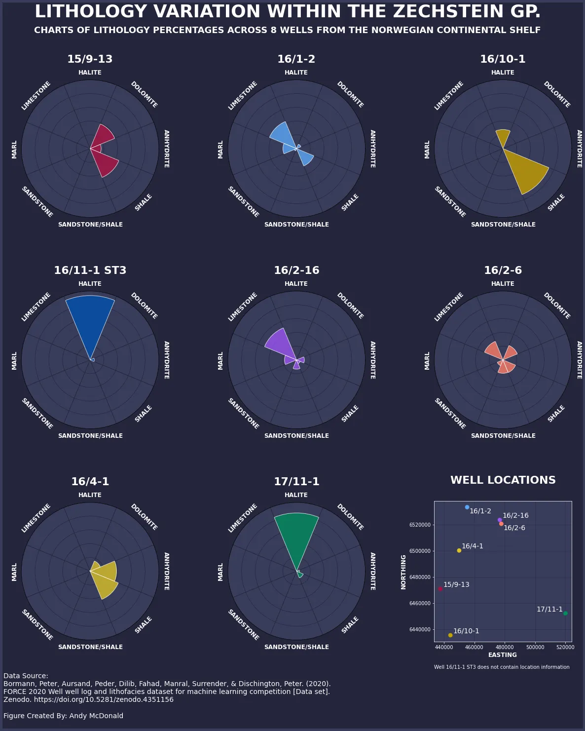
plt.suptitle('LITHOLOGY VARIATION WITHIN THE ZECHSTEIN GP.', measurement=36, fontweight='daring', shade='white')
plot_sub_title = """CHARTS OF LITHOLOGY PERCENTAGES ACROSS 8 WELLS FROM THE NORWEGIAN CONTINENTAL SHELF"""
fig.textual content(0.5, 0.95, plot_sub_title, ha='heart', va='high', fontsize=18, shade='white', fontweight='daring')
fig.textual content(0.1, 0.01, footnote, ha='left', va='backside', fontsize=14, shade='white')
plt.present()

After ending the plotting code, we’ll find yourself with a matplotlib determine just like the one beneath.

We have now all of the radial bar charts on show and the place every of the wells is situated. This enables the reader to know any spatial variation between the wells, which in flip might assist clarify variances throughout the knowledge.

For instance, Properly 15/9–13 is situated on the world’s western aspect and consists of a mix of dolomite, anhydrite and shale. Whereas effectively 17/11–1 is situated on the easter aspect of the world and is predominantly composed of halite. This could possibly be attributable to completely different depositional environments throughout the area.

The complete code for the infographic is displayed beneath, with every of the primary sections commented.

# Set the variety of columns to your subplot grid
num_cols = 3
# Get the variety of wells (rows within the DataFrame)
num_wells = len(df)
# Calculate the variety of rows wanted for the subplot grid
num_rows = np.ceil(num_wells / num_cols).astype(int)
indexes = record(vary(0, len(lith_names)))
width = 2*np.pi / len(lith_names)
angles = [element * width for element in indexes]
colors = ["#ae1241", "#5ba8f7", "#c6a000", "#0050ae", "#9b54f3", "#ff7d67", "#dbc227", "#008c5c"]
label_loc = np.linspace(begin=0, cease=2 * np.pi, num=len(lith_names))
# Create a determine
fig = plt.determine(figsize=(20, num_rows * 7), linewidth=10,
edgecolor='#393d5c', 
facecolor='#25253c')
# Create a grid structure
grid = plt.GridSpec(num_rows, num_cols, wspace=0.5, hspace=0.5)
# Loop over every row within the DataFrame to create the radial bar charts per effectively
for i, (index, row) in enumerate(df.iterrows()):
ax = fig.add_subplot(grid[i // num_cols, i % num_cols], projection='polar')
bars = ax.bar(x=angles, peak=row.values, width=width, 
edgecolor='white', zorder=2, alpha=0.8, shade=colors[i])
bars_bg = ax.bar(x=angles, peak=100, width=width, shade='#393d5c',
edgecolor='#25253c', zorder=1)
# Arrange labels, ticks and grid
ax.set_title(index, pad=35, fontsize=22, fontweight='daring', shade='white')
ax.set_ylim(0, 100)
ax.set_yticklabels([])
ax.set_xticks([])
ax.grid(shade='#25253c')
#Arrange the lithology / class labels to look on the appropriate angle
for angle, peak, lith_name in zip(angles, row.values, lith_names):
rotation_angle = np.levels(angle)
if angle < np.pi:
rotation_angle -= 90
elif angle == np.pi:
rotation_angle -= 90
else:
rotation_angle += 90
ax.textual content(angle, 110, lith_name.higher(), 
ha='heart', va='heart', 
rotation=rotation_angle, rotation_mode='anchor', fontsize=12, 
fontweight='daring', shade='white')
# Add the scatter plot within the final subplot (subplot 9)
ax = fig.add_subplot(grid[num_rows - 1, num_cols - 1], facecolor='#393d5c')
ax.scatter(zechstein_well_intersections['X_LOC'], zechstein_well_intersections['Y_LOC'], c=colors, s=60)
ax.grid(alpha=0.5, shade='#25253c')
ax.set_axisbelow(True)
# Arrange the labels and ticks for the scatter plot
ax.set_ylabel('NORTHING', fontsize=12, 
fontweight='daring', shade='white')
ax.set_xlabel('EASTING', fontsize=12, 
fontweight='daring', shade='white')
ax.tick_params(axis='each', colours='white')
ax.ticklabel_format(type='plain')
ax.set_title('WELL LOCATIONS', pad=35, fontsize=22, fontweight='daring', shade='white')
# Set the surface borders of the scatter plot to white
ax.spines['bottom'].set_color('white')
ax.spines['top'].set_color('white') 
ax.spines['right'].set_color('white')
ax.spines['left'].set_color('white')
# Add a footnote to the scatter plot explaining lacking effectively
ax.textual content(0.0, -0.2, 'Properly 16/11-1 ST3 doesn't comprise location data', ha='left', va='backside', fontsize=10,
shade='white', rework=ax.transAxes)
# Arrange and show effectively identify labels
labels = []
for i, row in zechstein_well_intersections.iterrows():
labels.append(ax.textual content(row['X_LOC'], row['Y_LOC'], row['WELL'], shade='white', fontsize=14))
# Use modify textual content to make sure textual content labels don't overlap with one another or the info factors
adjust_text(labels, expand_points=(1.2, 1.2), expand_objects=(1.2, 1.2))
# Create a footnote explaining knowledge supply
footnote = """
Knowledge Supply: 
Bormann, Peter, Aursand, Peder, Dilib, Fahad, Manral, Give up, & Dischington, Peter. (2020). FORCE 2020 Properly effectively log and lithofacies dataset for
machine studying competitors [Data set]. Zenodo. https://doi.org/10.5281/zenodo.4351156
Determine Created By: Andy McDonald
"""
# Show general infographic title and footnote
plt.suptitle('LITHOLOGY VARIATION WITHIN THE ZECHSTEIN GP.', measurement=36, fontweight='daring', shade='white')
plot_sub_title = """CHARTS OF LITHOLOGY PERCENTAGES ACROSS 8 WELLS FROM THE NORWEGIAN CONTINENTAL SHELF"""
fig.textual content(0.5, 0.95, plot_sub_title, ha='heart', va='high', fontsize=18, shade='white', fontweight='daring')
fig.textual content(0.1, 0.01, footnote, ha='left', va='backside', fontsize=14, shade='white')
plt.present()

Infographics are a good way to summarise knowledge and current it to readers in a compelling and attention-grabbing approach with out them having to fret concerning the uncooked numbers. It is usually a good way to inform tales about your knowledge.

At first, chances are you’ll not suppose matplotlib is equipped for creating infographics, however with some observe, effort and time, it’s undoubtedly attainable.

Coaching dataset used as a part of a Machine Studying competitors run by Xeek and FORCE 2020 (Bormann et al., 2020). This dataset is licensed underneath Artistic Commons Attribution 4.0 Worldwide.

The complete dataset might be accessed on the following hyperlink: https://doi.org/10.5281/zenodo.4351155.